Scatter or dot plots
There are two sets of scatter plot functions that use either geom_dotplot (i.e. plot_dot.. functions) or geom_point (i.e. plot_scatter..) geometries from ggplot2. When a lot of data points are involved, use plot_scatter.. functions and reduce overlap by increasing the value of the jitter argument.
Common arguments
All plot_ functions require a long-format data table as the first argument, followed by the name of the column (a categorical variable) to be plotted on the X-axis (xcol) and the quantitative variable to be plotted on the Y-axis (ycol). If provided in this order the data =, xcol = and ycol = need not be explicitly called (see examples below).
The next argument is facets, which enables the addition of another variable if necessary.
NOTE: in several examples below I’ve added guides(fill = "none") to save space; legends will be shown as default.
Data format
See the data help page and ensure data table is in the long-format.
Saving graphs
See Saving graphs for tips on how to save plots for making figures.
Bar graphs
plot_scatterbar_sd & plot_dotbar_sd
These functions plot bar graphs and show all data as scattered symbols for data (also called jittered symbols) using two kinds of layouts. In both cases, the categorical X variable is also mapped to the fill aesthetic for bars and symbols, and their colour can be set with ColPal argument.
Optional arguments include bsize (for bar width), ewid (error bar width), and symsize or dotsize (symbol or dot size, respectively). Opacity of bars and symbols can be set independently using b_alpha and s_alpha arguments, respectively. (Until v0.3.1, there was only a single alpha parameter to set the opacity of symbols. Older code with alpha will break v1.4.1, sorry!)
#scatterbar
plot_scatterbar_sd(data = data_1w_death, #data table
xcol = Genotype, #X variable
ycol = Death, #Y variable
fontsize = 25)+
labs(title = "Scatter dots with bar & SD", #title
subtitle = "(default `okabe_ito` palette)")+
guides(fill = "none")
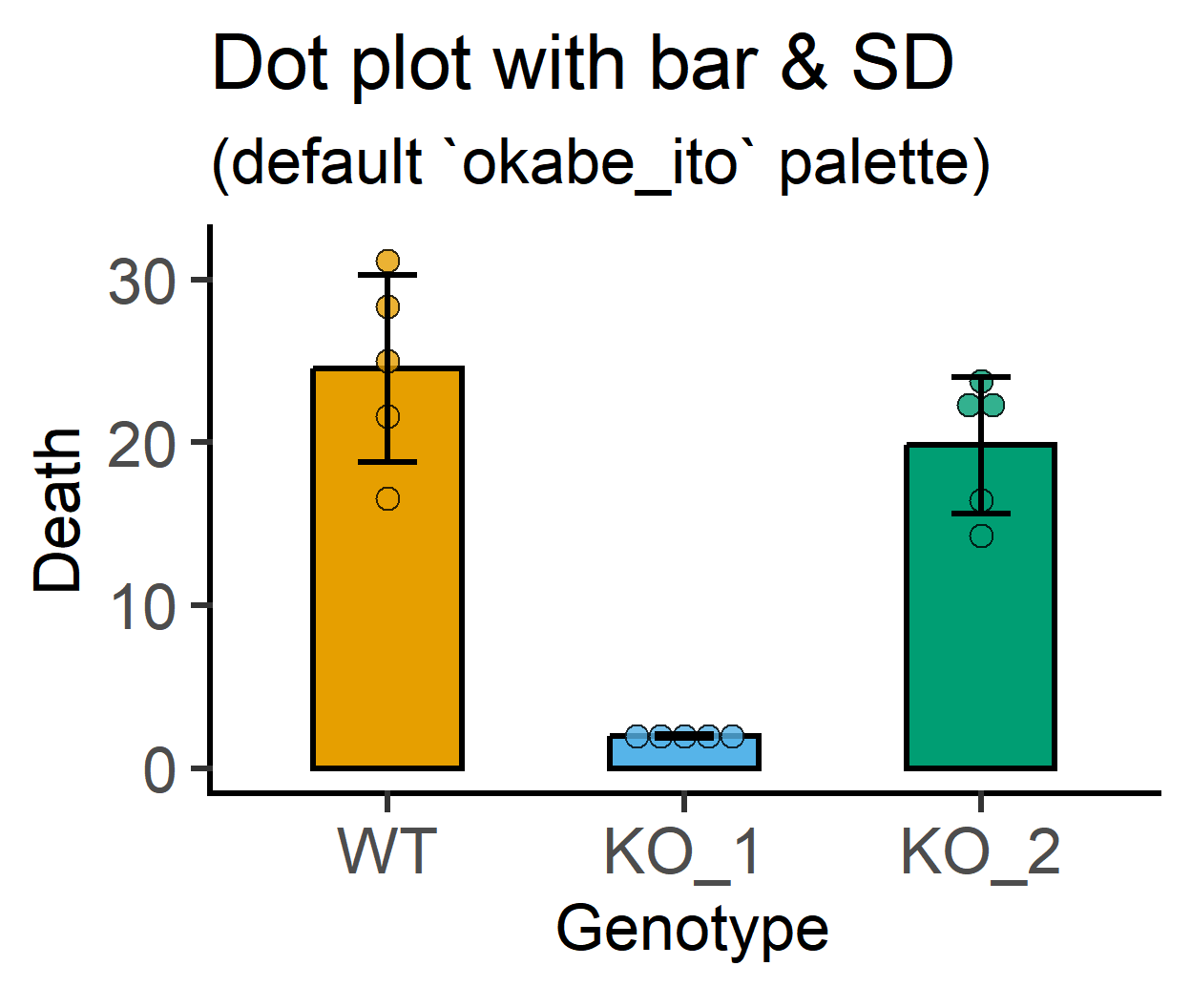
#scatterbar
plot_dotbar_sd(data = data_1w_death, #data table
xcol = Genotype, #X variable
ycol = Death, #Y variable
fontsize = 25)+
labs(title = "Dot plot with bar & SD", #title
subtitle = "(default `okabe_ito` palette)")+
guides(fill = "none")
symsize and ewid for symbol size and error bar width
#larger symbols
plot_scatterbar_sd(data_1w_death,
Genotype,
Death,
symsize = 4)+ #larger symbol size
labs(title = "Larger symbols")+
guides(fill = "none")
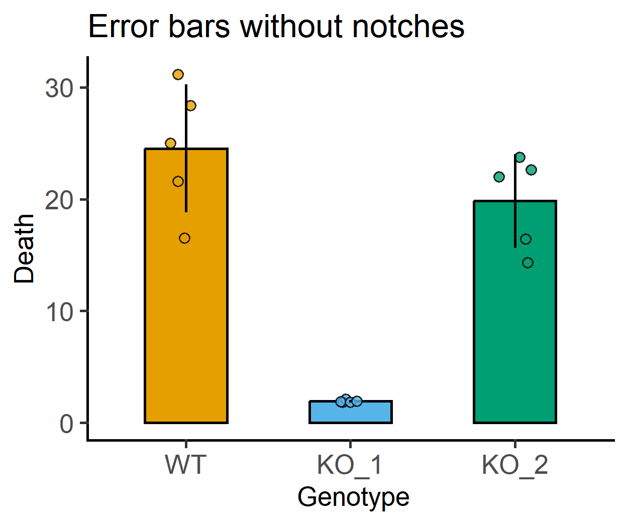
#error bars without notches
plot_scatterbar_sd(data_1w_death,
Genotype,
Death,
ewid = 0)+ #error bars without notches
labs(title = "Error bars without notches")+
guides(fill = "none")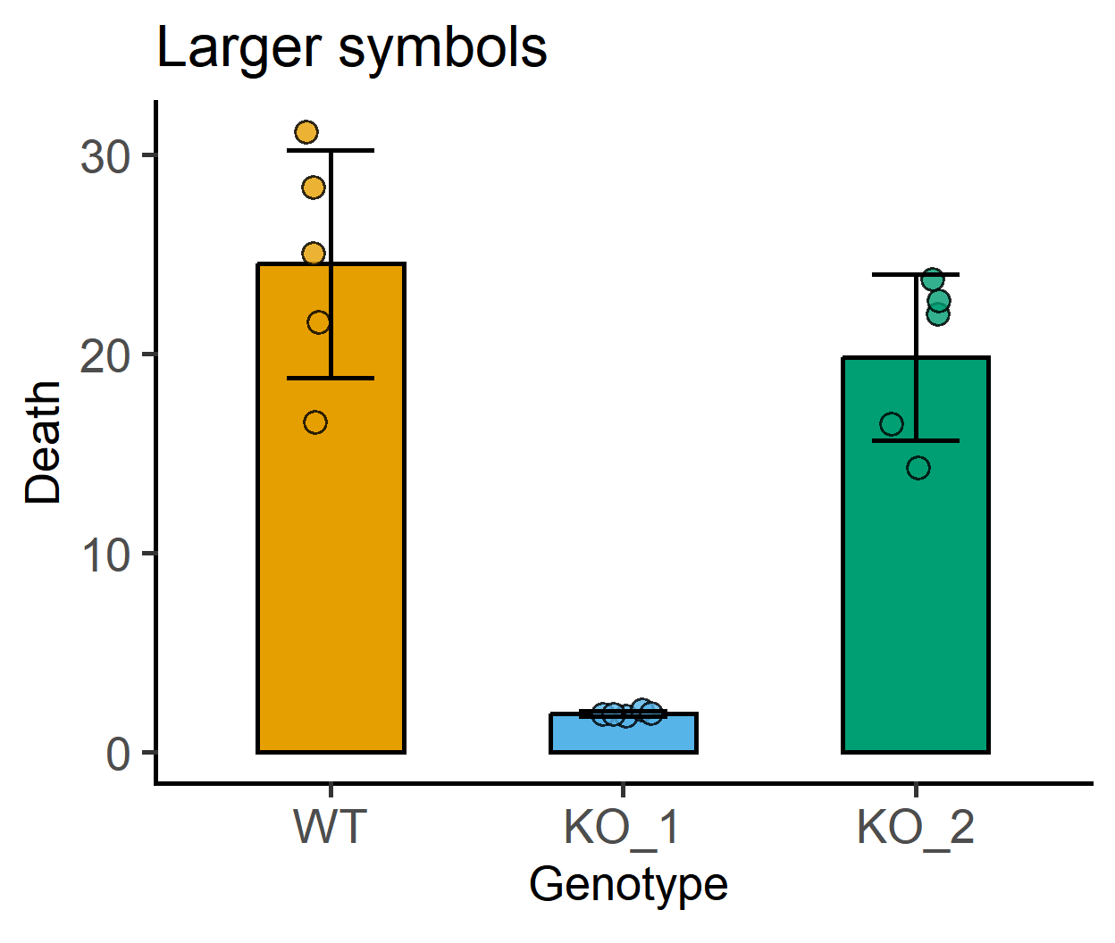
ColPal, ColRev and ColSeq for colours
Let’s first see the colour order in okabe_ito and vibrant palettes.
#default palette (okabe_ito)
plot_grafify_palette("okabe_ito", fontsize = 25)+
labs(title = "okabe_ito")
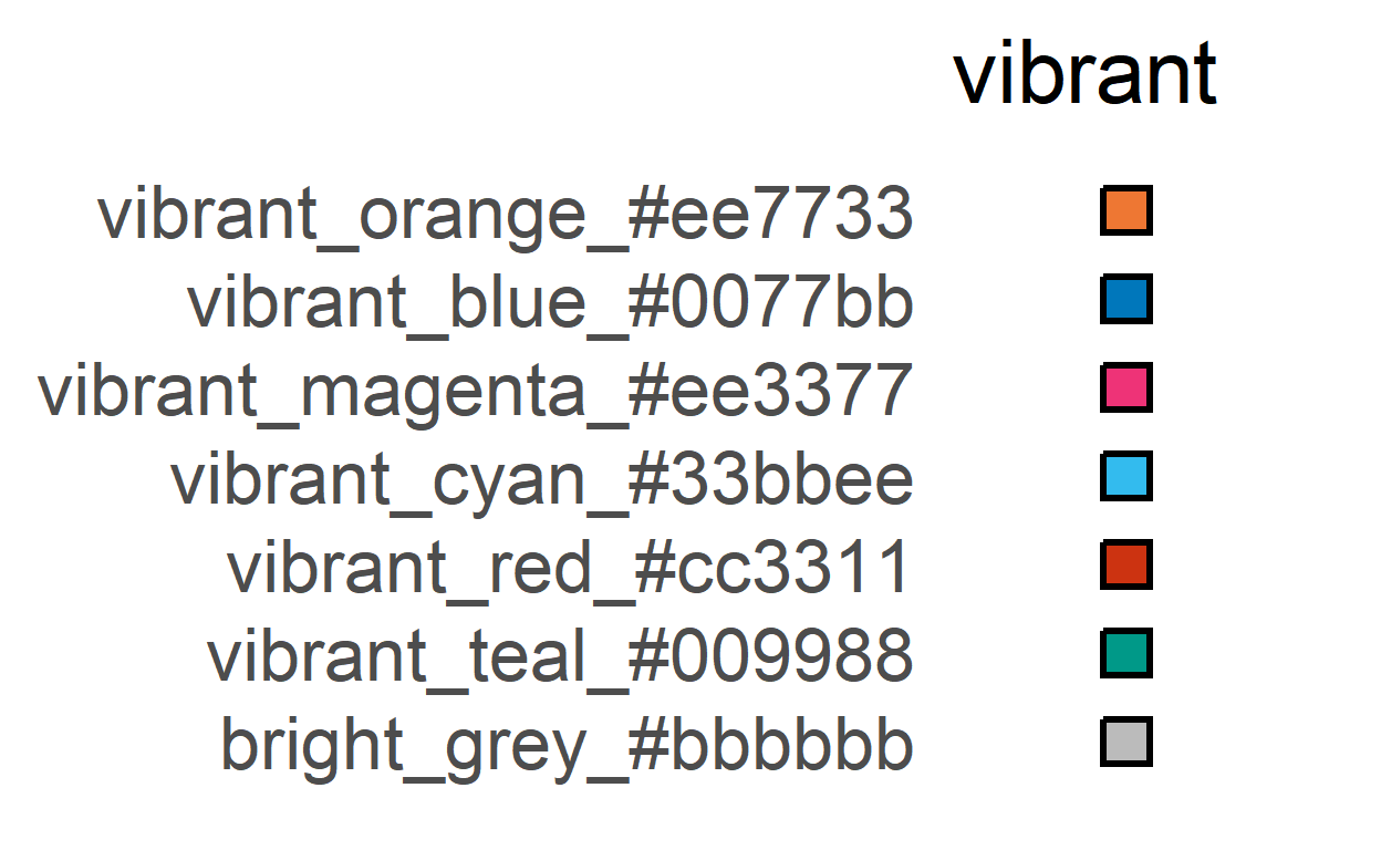
#choose a different one
plot_grafify_palette("vibrant", fontsize = 25)+
labs(title = "vibrant")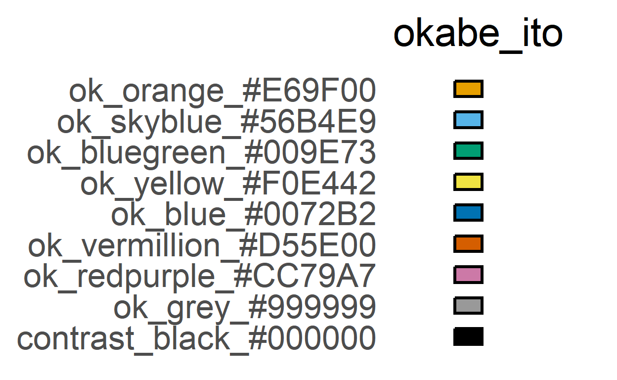
Let’s change colour palette and order of colours.
#change to `vibrant` palette
plot_scatterbar_sd(data_1w_death, #data table
Genotype, #X variable
Death,
symsize = 3, fontsize = 25,
ColPal = "vibrant", #vibrant palette
TextXAngle = 45)+ #rotate text 45 deg
labs(title = "`vibrant` palette")+ #subtitle
guides(fill = "none") #no legend
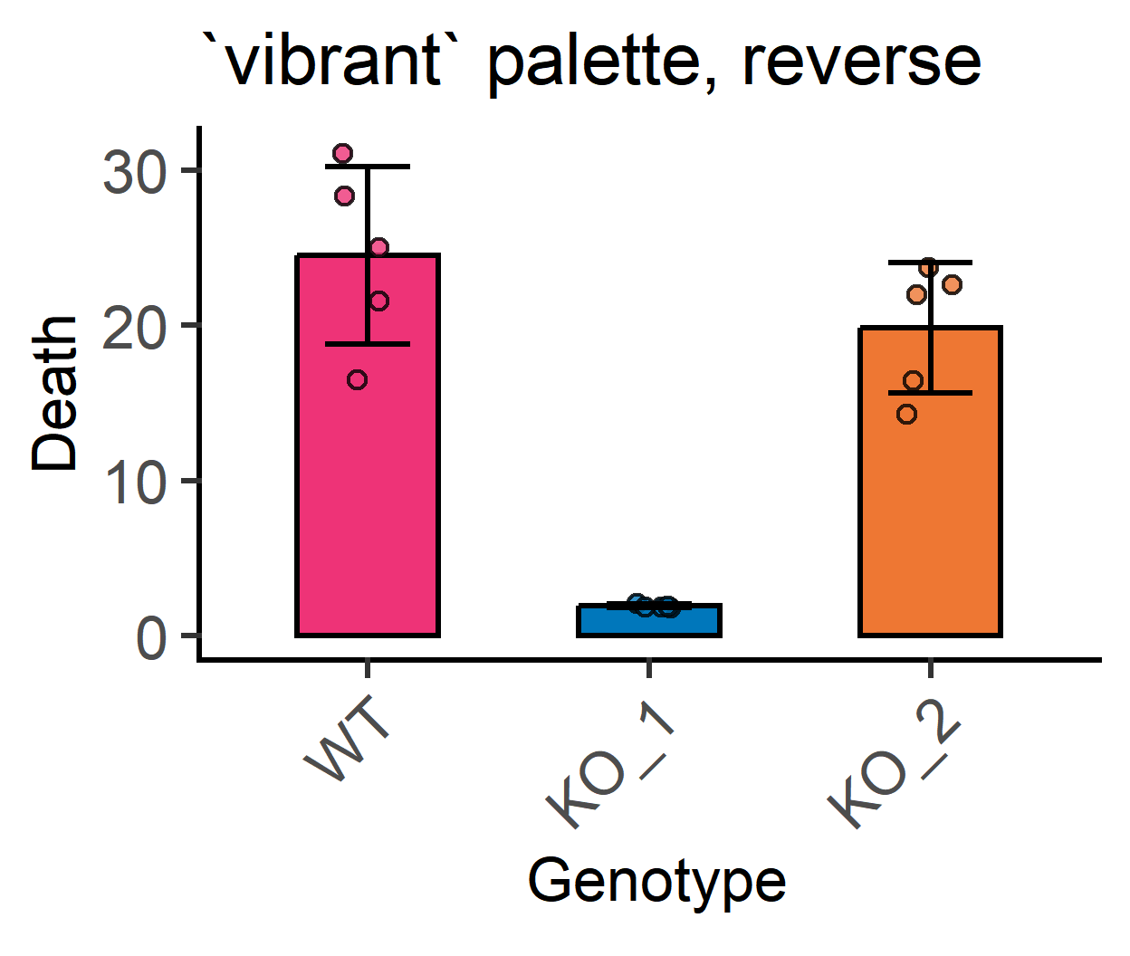
#reverse colours from `vibrant` palette
plot_scatterbar_sd(data_1w_death, #data table
Genotype, #X variable
Death,
symsize = 3, fontsize = 25,
ColPal = "vibrant", #vibrant palette
ColRev = T, #reverse palette
TextXAngle = 45)+ #rotate text 45 deg
labs(title = "`vibrant` palette, reverse")+ #subtitle
guides(fill = "none") #no legend
#reverse colours from `vibrant` palette
plot_scatterbar_sd(data_1w_death, #data table
Genotype, #X variable
Death,
symsize = 3, fontsize = 25,
ColPal = "vibrant", #vibrant palette
ColSeq = F, #not sequential colours
TextXAngle = 45)+ #rotate text 45 deg
labs(title = "`vibrant` palette, distant colours")+ #subtitle
guides(fill = "none") #no legend
#reverse & distant colours from `vibrant` palette
plot_scatterbar_sd(data_1w_death, #data table
Genotype, #X variable
Death,
symsize = 3, fontsize = 25,
ColPal = "vibrant", #vibrant palette
ColRev = T, #reverse
ColSeq = F, #not sequential colours
TextXAngle = 45)+ #rotate text 45 deg
labs(title = "`vibrant`, rev, distant colours")+ #subtitle
guides(fill = "none") #no legend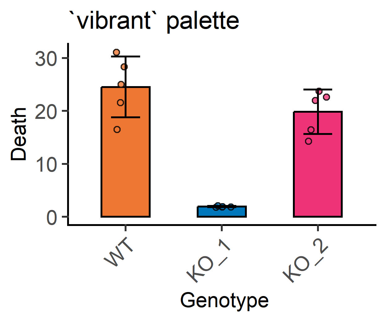


s_alpha & b_alpha for symbol or bar opacity
For plot_scatter... functions, symbol opacity is set using s_alpha argument, and in plot_dot... this is adjusted via the d_alpha argument. Opacity of bar, box or violins is adjusted with b_alpha or v_alpha. This example makes bars white (b_alpha = 0), increases jitter to reduce symbol overlap and also reduces symbol opacity s_alpha = 0.7
#transparent bars
plot_scatterbar_sd(data_1w_death,
Genotype,
Death,
symsize = 3, fontsize = 25,
b_alpha = 0)+ #completely transparent
labs(title = "transparent bars")+ #subtitle
guides(fill = "none")
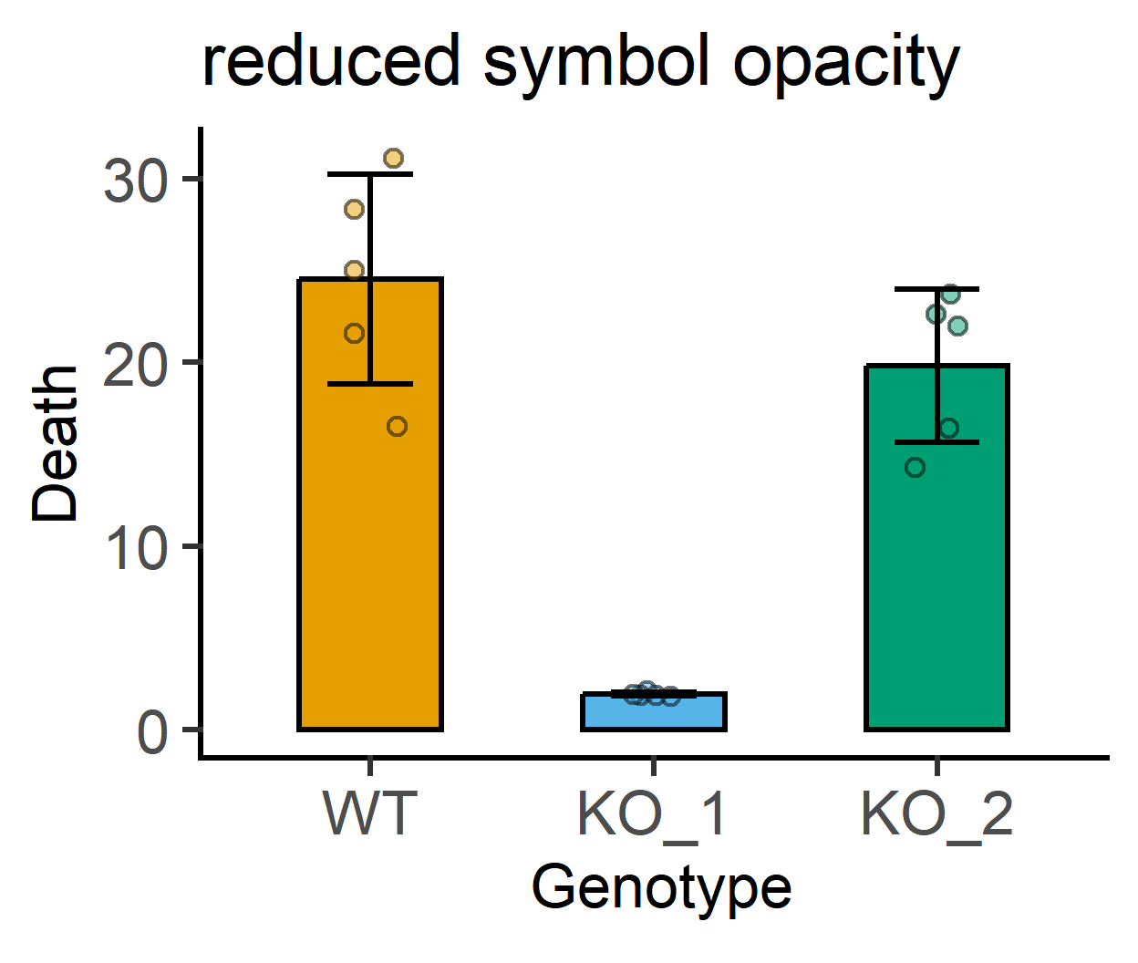
#increased symbol transparency
plot_scatterbar_sd(data_1w_death,
Genotype,
Death,
symsize = 3, fontsize = 25,
s_alpha = 0.5)+ #symbol transparency
labs(title = "reduced symbol opacity")+ #subtitle
guides(fill = "none")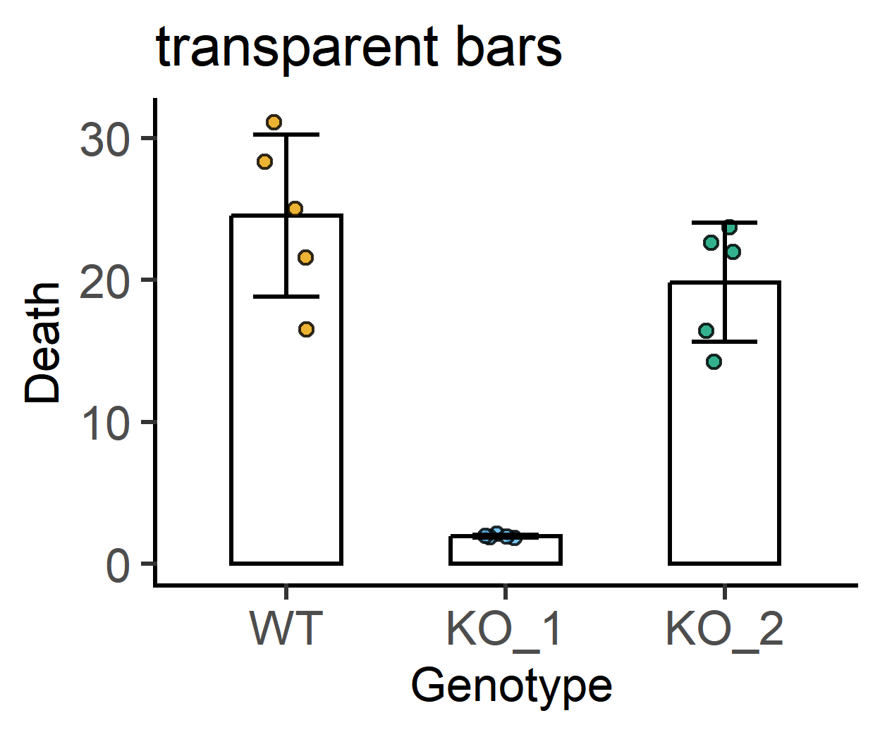
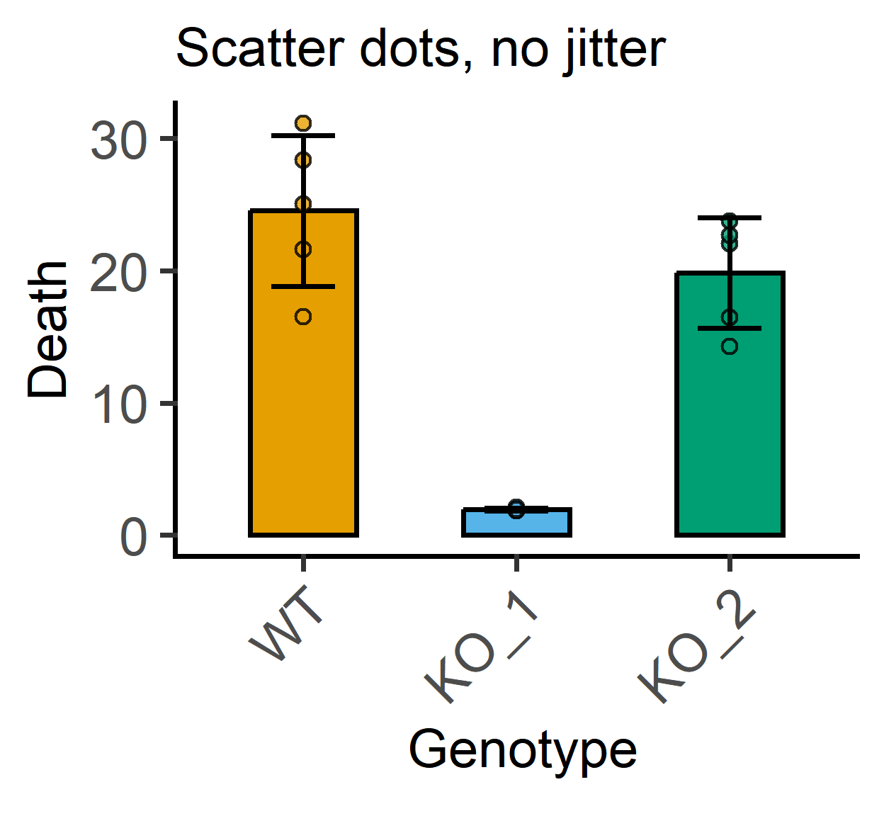
jitter for symbol scatter
This can be done for all plot_scatter... functions (but not plot_dot... where layout is set automatically to prevent overlap of symbols).
plot_scatterbar_sd(data_1w_death,
                   Genotype,
                   Death,
                   symsize = 3, fontsize = 28,
                   TextXAngle = 45)+  #rotate text 45 deg
  labs(subtitle = "Scatter dots, default jitter")+ #subtitle
  guides(fill = "none")
#no jitter
plot_scatterbar_sd(data_1w_death,
                   Genotype,
                   Death,
                   symsize = 3, fontsize = 28,
                   jitter = 0,   #no jitter
                   TextXAngle = 45)+  #rotate text 45 deg
  labs(subtitle = "Scatter dots, no jitter")+ #subtitle
guides(fill = "none") 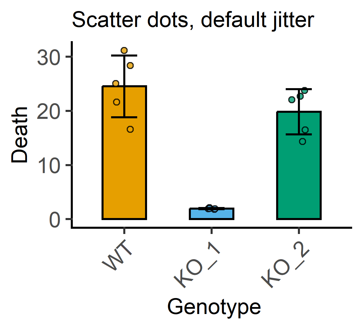
plot_dotbar_sd
This is similar to plot_scatterbar_sd, but uses geom_dotplot instead of geom_point, which can sometimes generate a ‘cleaner’ layout. Optional settings include dotsize, ewid and fontsize, which change the relative size of dots, error bar width and base font size. Here too, the categorical X variable is mapped to the fill aesthetic of the dots and the bar. Advanced parameters can also be set (look into ?geom_dotplot for help.)
For plot_dot... functions, symbol opacity is set using d_alpha argument (and bar, box or violin opacity with b_alpha or v_alpha).
Binsize in dotplots
Some dot plots may need an adjustment of the binwidth argument of geom_dotplot geometry, which by ggplot2 default is Y axis range/30. This can be changed if necessary.
Box and whiskers plots
plot_scatterbox and plot_dotbox
These related functions generate showing all data layered on top of a box and whiskers plot. The categorical X variable is mapped to the fill aesthetic of symbols and boxes.
In the boxplot, the thick line is the median, the box itself covers the interquantile range (IQR), and the whiskers indicate 1.5x IQR.
The default size of dots can be changed with dotsize and symbols with symsize, respectively.
Advanced parameters can also be set (look into ?geom_boxplot for help.)
plot_scatterbox(data_1w_death, #data table
Genotype, #X variable
Death, #Y variable
symsize = 5, fontsize = 25,
jitter = 0.2)+ #jitter
labs(title = "Scatter & boxplot")+
guides(fill = "none")
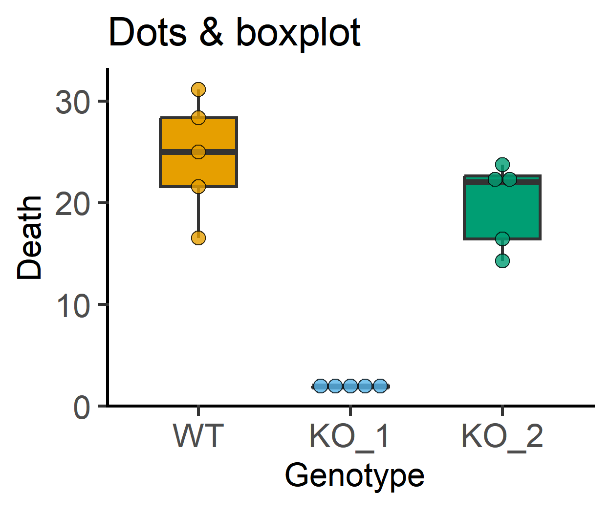
plot_dotbox(data_1w_death, #data table
Genotype, #X variable
Death, #Y variable
dotsize = 1.5, fontsize = 25)+
labs(title = "Dots & boxplot")+
guides(fill = "none")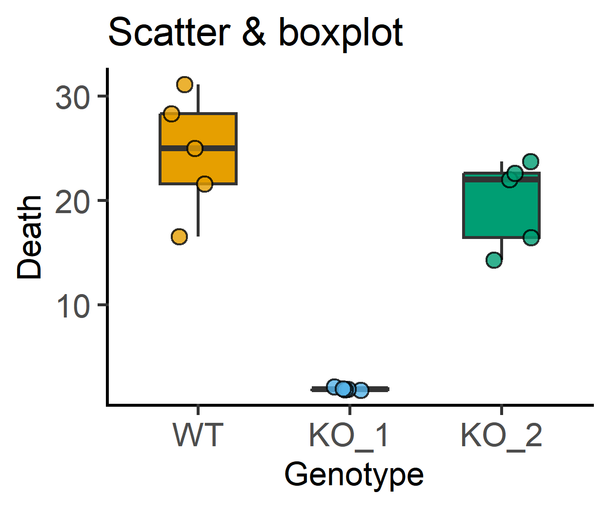
b_alpha for transparent boxes
plot_scatterbox(data_t_pratio, #data table
                Genotype,      #X variable
                Cytokine,      #Y variable
                ColPal = "muted",
                jitter = 0.1,  #symbol jitter
                s_alpha = 0.7, #symbol opacity
                b_alpha = 0,   #box opacity
                LogYTrans = "log10")+ #transform Y axis

  labs(title = "Scatter & box plot, `muted` palette",
       subtitle = "jitter & bar opacity")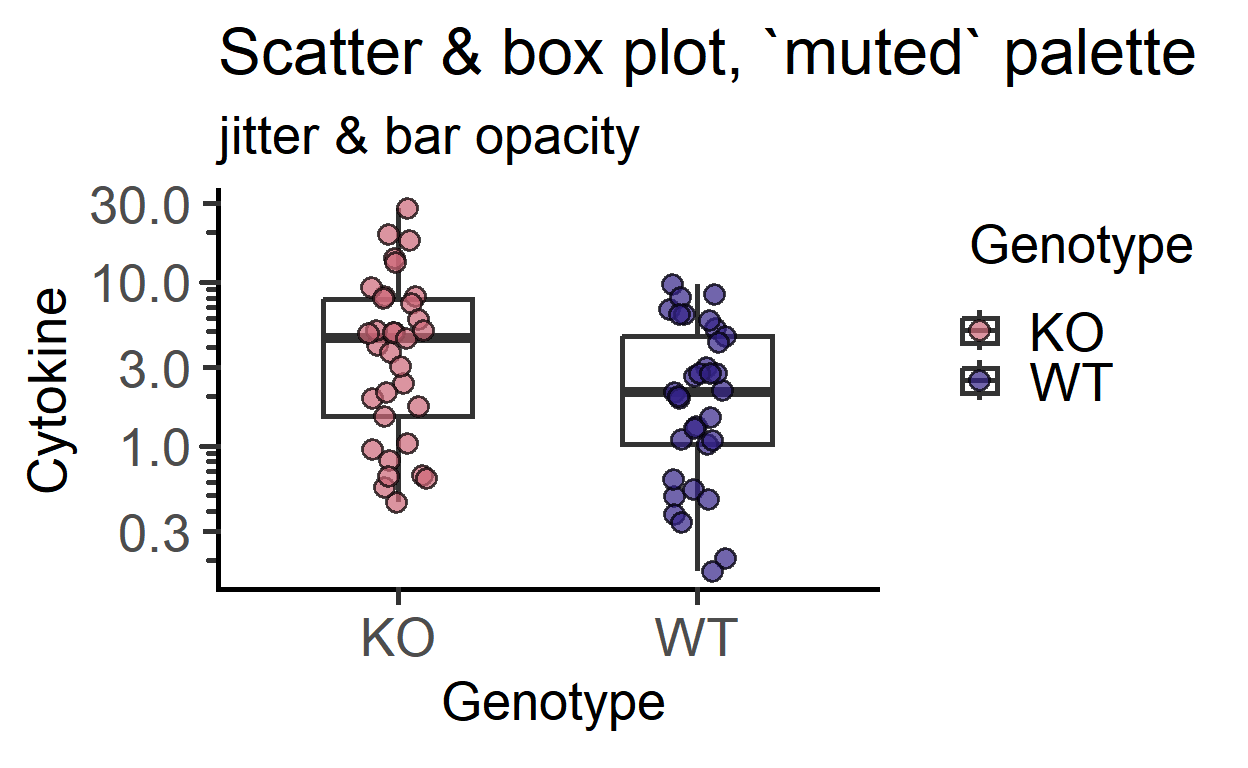
Violin plots
plot_scatter_violin and plot_dot_violin
These take similar arguments as boxplot functions above but plot a violin plot instead. Here’s an example of a violin plot with defaults. Since v2.0.0, a box and whiskers plot is also plotted on top of the violin. The box plot shows median and IQR, whiskers depict 1.5*IQR.
plot_dotviolin(data_t_pratio, #data table
Genotype, #X variable
Cytokine, #Y variable
fontsize = 25,
ColPal = "pale", #"pale" palette
LogYTrans = "log10")+ #log10 transform
labs(title = "Dots & violin plot, `pale`",
subtitle = "default (trim = F)")+
guides(fill = "none")
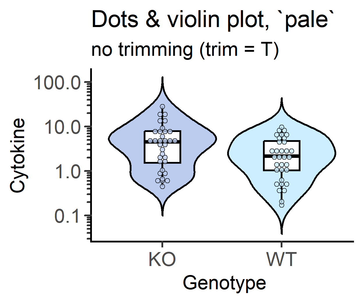
#no trimming
plot_dotviolin(data_t_pratio, #data table
Genotype, #X variable
Cytokine, #Y variable
trim = FALSE, #no trimming
fontsize = 25,
ColPal = "pale", #"pale" palette
LogYTrans = "log10")+ #log10 transform
labs(title = "Dots & violin plot, `pale`",
subtitle = "no trimming (trim = T)")+
guides(fill = "none")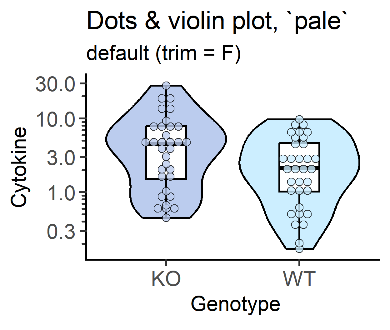
v_alpha & b_alpha for violin opacity
An example with transparent violins with just the symbols showing colour.
plot_scatterviolin(data_t_pratio, #data table
Genotype, #X variable
Cytokine, #Y variable
ColPal = "muted", fontsize = 25,
jitter = 0.1, #symbol jitter
s_alpha = 0.7, #symbol opacity
v_alpha = 0, #violin opacity
trim = F, #trim set to false
LogYTrans = "log10")+ #log10 transform)
labs(title = "transparent violins")+
guides(fill = "none")
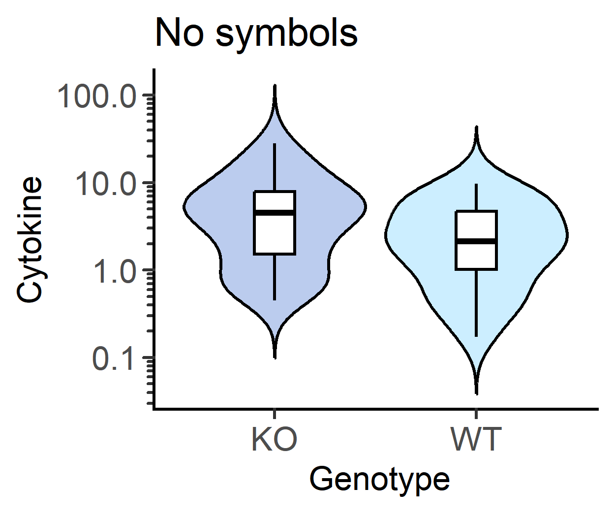
#symbol opacity
plot_scatterviolin(data_t_pratio, #data table
Genotype, #X variable
Cytokine, #Y variable
ColPal = "pale", fontsize = 25,
jitter = 0.2, #symbol jitter
s_alpha = 0, #symbol opacity
bwid = 0.2, #width of boxplot
trim = F, #trim set to false
LogYTrans = "log10")+ #log10 transform)
labs(title = "No symbols")+
guides(fill = "none")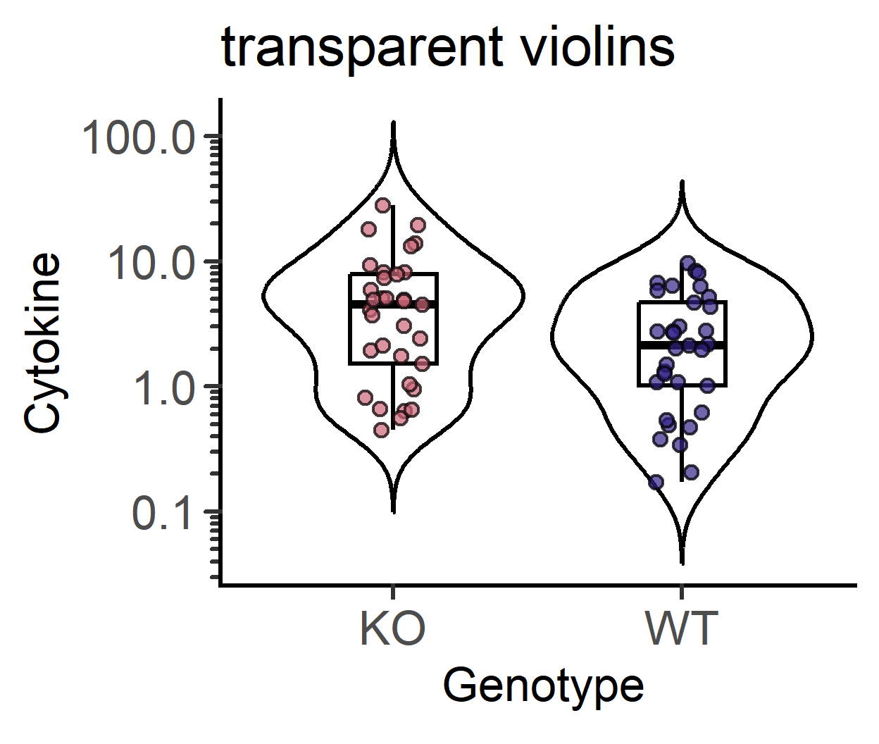
b_alpha for white boxplots inside violins
The default is b_alpha = 0, which results in a white boxplot irrespective of palette chosen for violins. This can be changed by setting a different value for b_alpha.
plot_scatterviolin(data_t_pratio, #data table
Genotype, #X variable
Cytokine, #Y variable
ColPal = "pale", fontsize = 25,
jitter = 0.2, #symbol jitter
s_alpha = 0, #symbol opacity
LogYTrans = "log10")+ #log10 transform)
labs(title = "white boxes")+
guides(fill = "none")
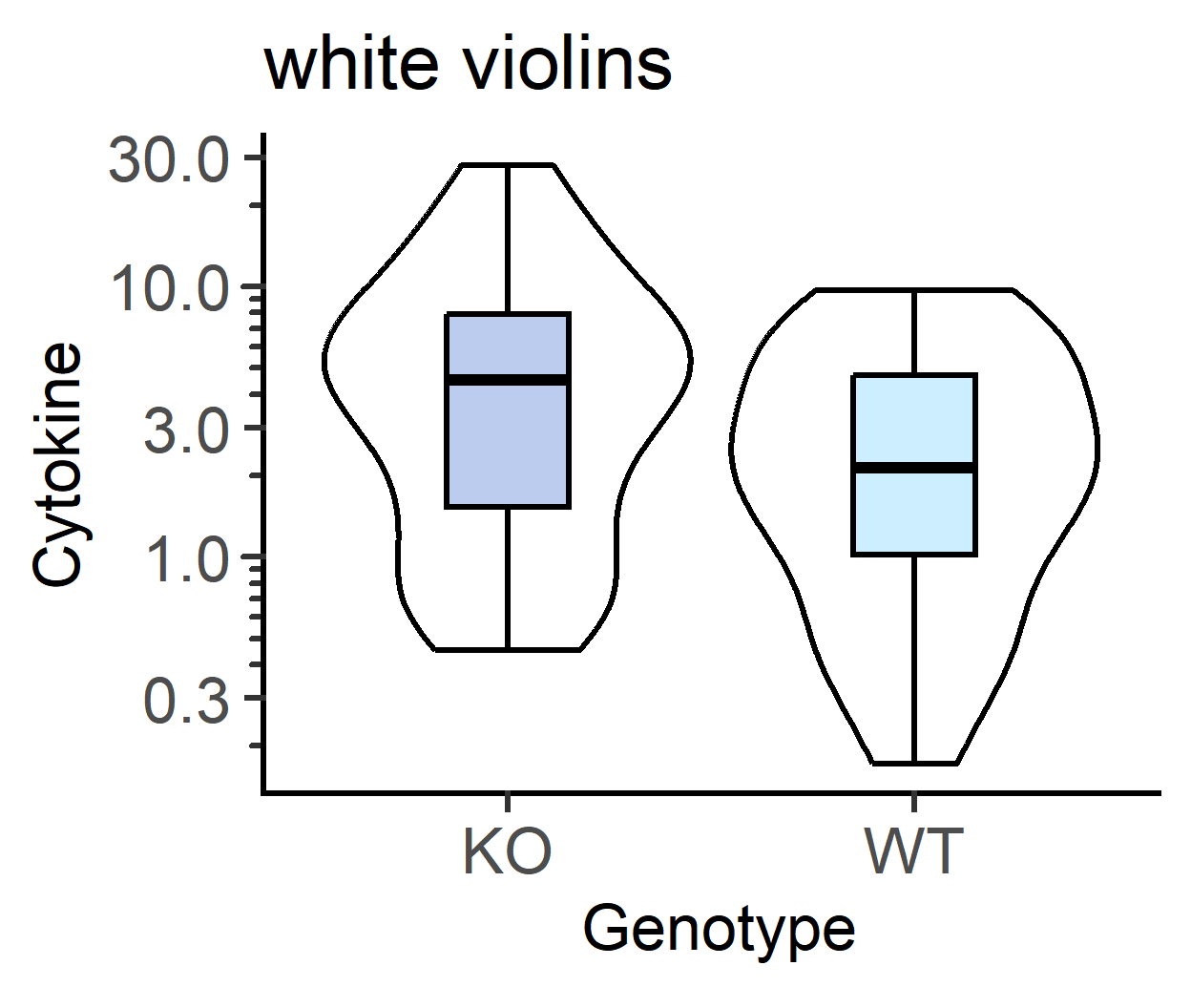
#white violins, coloured boxes
plot_scatterviolin(data_t_pratio, #data table
Genotype, #X variable
Cytokine, #Y variable
ColPal = "pale", fontsize = 25,
jitter = 0.2, #symbol jitter
s_alpha = 0, #symbol opacity
v_alpha = 0, #transparent violins
b_alpha = 1, #opaque boxes
LogYTrans = "log10")+ #log10 transform
labs(title = "white violins")+
guides(fill = "none")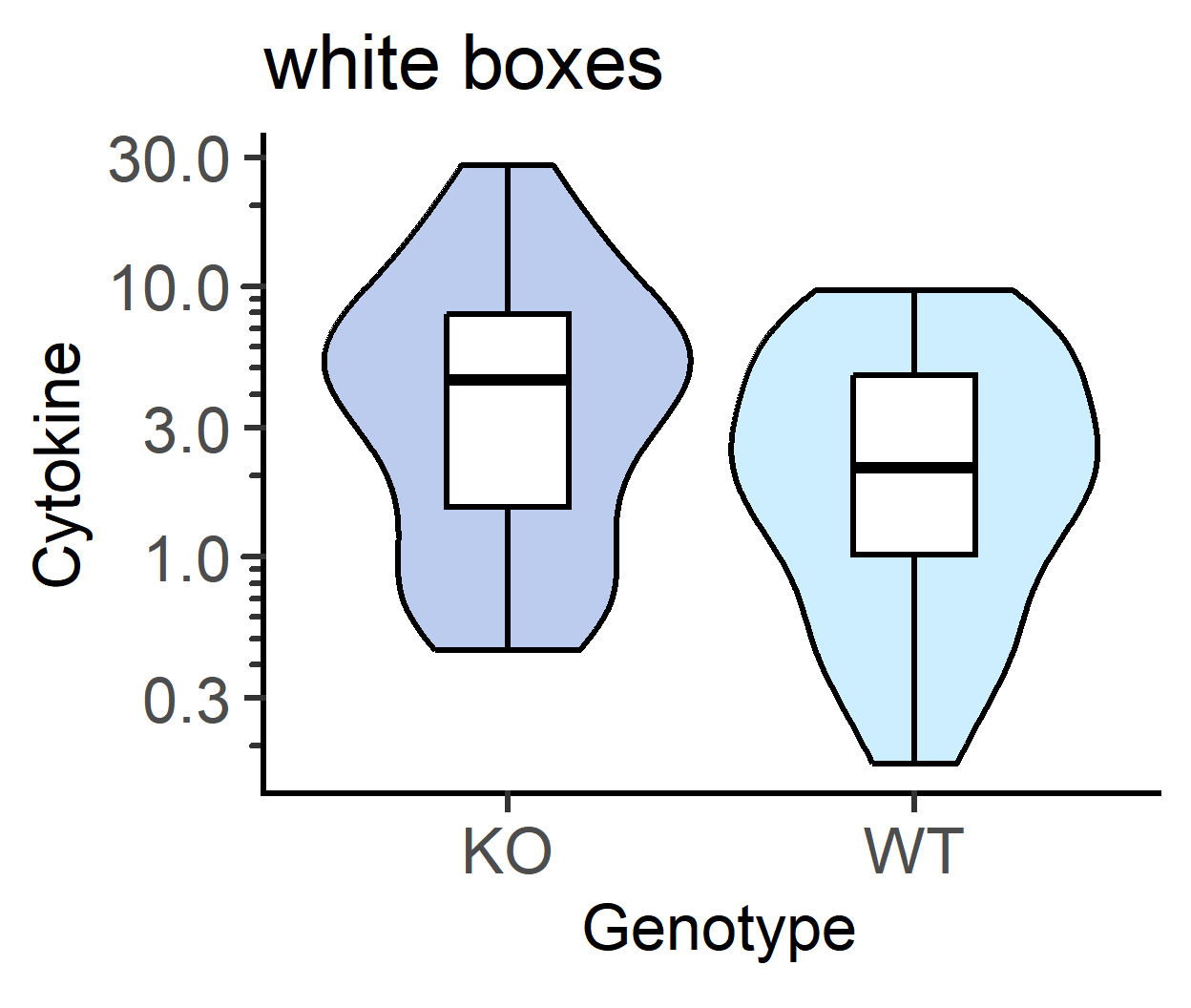
Summary bar/point with SD
These are generally not recommended as it is best to show all data values.
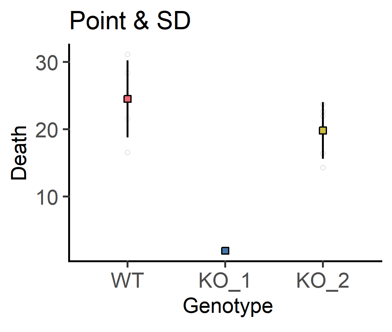
plot_point_sd
By default, this function depicts mean and SD, which is less recommended as it is best to show all data whenever possible. in v3.1.0, all data points can be shown using opacity parameter all_alpha (which is set to 0 by default). The size, shape and jitter of all data points can be adjusted with all_size, all_shape and all_jitter, respectively. The symsize and ewid arguments set the symbol size and width of error bars, respectively.
The categorical X variable is mapped to the fill aesthetic of the bar and points.
The plot_bar_sd function is now deprecated; use plot_scatterbar_sd with s_alpha = 0 if you need it.
plot_point_sd(data_1w_death,
Genotype,
Death,
ColPal = "bright",
fontsize = 25,
ewid = 0)+ #no width on SD error bar
labs(title = "Point & SD")+
guides(fill = "none")
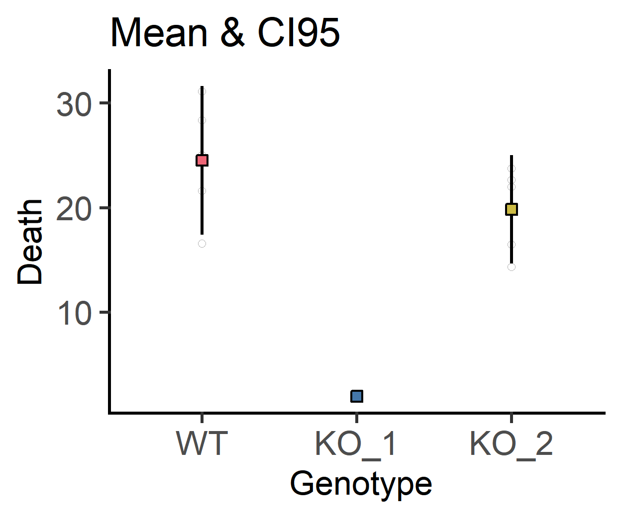
#show all data
plot_point_sd(data_1w_death,
Genotype,
Death,
all_alpha = 0.5, #opacity of all data
all_jitter = 0.1, #jitter for all data
ColPal = "bright",
fontsize = 25,
ewid = 0)+ #no width on SD error bar
labs(title = "Mean & SD")+
guides(fill = "none")
#CI95 error bars
plot_point_sd(data_1w_death,
Genotype,
Death,
ErrorType = "CI95", #CI95 error bars
ColPal = "bright",
fontsize = 25,
ewid = 0)+ #no width on SD error bar
labs(title = "Mean & CI95")+
guides(fill = "none")