grafify includes the following functions for post-hoc comparisons:
posthoc_Pariwise: all-vs-all comparisonsposthoc_Levelwise: level-wise within a factorposthoc_vsRef: compare against a control or reference group
All of these are based on the emmeans package. The output has two sections, $emmeans (estimated marginal means) which lists the emmeans, upper and lower CI95 and degrees of freedom, and $contrasts which lists the post-hoc comparisons with key details such as the SE, t ratio and P value. posthoc_ functions need the linear model fit using simple_model or mixed_model, and fixed factors(s) whose levels you wish to compare, which should match those used for fitting the model. For this vignette, I’ll first save models fitted with using simple_model and mixed_model to illustrate posthoc_ functions.
library(grafify)
library(emmeans)
library(boot)   #for logit transformation

#simple model
sm_dtime <- simple_model(data_doubling_time, #data table
                         "Doubling_time",    #dependent variable
                         "Student")          #one fixed factor

#mixed model with one random factor
mod_chol <- mixed_model(data_cholesterol,    #data table
                        "Cholesterol",       #dependent variable
                        c("Hospital", "Treatment"),  #two fixed factors
                        "Subject")           #random factor

#mided model with two random factors
mod_2wtdeath <- mixed_model(data_2w_Tdeath,
            "logit(PI/100)",     #logit transformation in formula
            c("Genotype", "Time"),           #two fixed factors
            c("Experiment", "Subject"))      #two random factors
posthoc_Pairwise
This will generate a lot of comparisons and should be used only when necessary. By default, multiple comparisons are corrected by the FDR method in grafify. This can be changed using the P_Adj argument.
As you will see with data from 10 students, pairwise comparisons generates a LOT of P values! Below I use the same model to compare every student with student A as Reference using posthoc_vsRef.
The essential arguments are the Model object and Factors which is a vector of fixed factors and should match those used in the Model object.
posthoc_Pairwise(sm_dtime,        #model fit with simple_model
                 "Student")       #fixed factor
#> $emmeans
#> Student emmean SE df lower.CL upper.CL
#> A 20.0 1.15 20 17.6 22.4
#> B 19.6 1.15 20 17.2 22.0
#> C 19.4 1.15 20 17.0 21.8
#> D 18.8 1.15 20 16.4 21.2
#> E 19.3 1.15 20 16.9 21.7
#> F 20.7 1.15 20 18.3 23.1
#> G 20.5 1.15 20 18.1 22.8
#> H 19.2 1.15 20 16.8 21.5
#> I 20.6 1.15 20 18.2 23.0
#> J 21.2 1.15 20 18.8 23.6
#>
#> Confidence level used: 0.95
#>
#> $contrasts
#> contrast estimate SE df t.ratio p.value
#> A - B 0.3713 1.62 20 0.229 0.9554
#> A - C 0.5929 1.62 20 0.365 0.9554
#> A - D 1.1728 1.62 20 0.722 0.9554
#> A - E 0.6286 1.62 20 0.387 0.9554
#> A - F -0.7416 1.62 20 -0.457 0.9554
#> A - G -0.4885 1.62 20 -0.301 0.9554
#> A - H 0.8083 1.62 20 0.498 0.9554
#> A - I -0.6775 1.62 20 -0.417 0.9554
#> A - J -1.2115 1.62 20 -0.746 0.9554
#> B - C 0.2216 1.62 20 0.136 0.9554
#> B - D 0.8014 1.62 20 0.493 0.9554
#> B - E 0.2572 1.62 20 0.158 0.9554
#> B - F -1.1130 1.62 20 -0.685 0.9554
#> B - G -0.8598 1.62 20 -0.529 0.9554
#> B - H 0.4370 1.62 20 0.269 0.9554
#> B - I -1.0488 1.62 20 -0.646 0.9554
#> B - J -1.5829 1.62 20 -0.975 0.9554
#> C - D 0.5798 1.62 20 0.357 0.9554
#> C - E 0.0356 1.62 20 0.022 0.9827
#> C - F -1.3346 1.62 20 -0.822 0.9554
#> C - G -1.0814 1.62 20 -0.666 0.9554
#> C - H 0.2154 1.62 20 0.133 0.9554
#> C - I -1.2704 1.62 20 -0.782 0.9554
#> C - J -1.8044 1.62 20 -1.111 0.9554
#> D - E -0.5442 1.62 20 -0.335 0.9554
#> D - F -1.9144 1.62 20 -1.179 0.9554
#> D - G -1.6612 1.62 20 -1.023 0.9554
#> D - H -0.3644 1.62 20 -0.224 0.9554
#> D - I -1.8503 1.62 20 -1.139 0.9554
#> D - J -2.3843 1.62 20 -1.468 0.9554
#> E - F -1.3702 1.62 20 -0.844 0.9554
#> E - G -1.1170 1.62 20 -0.688 0.9554
#> E - H 0.1798 1.62 20 0.111 0.9554
#> E - I -1.3061 1.62 20 -0.804 0.9554
#> E - J -1.8401 1.62 20 -1.133 0.9554
#> F - G 0.2532 1.62 20 0.156 0.9554
#> F - H 1.5500 1.62 20 0.954 0.9554
#> F - I 0.0642 1.62 20 0.040 0.9827
#> F - J -0.4699 1.62 20 -0.289 0.9554
#> G - H 1.2968 1.62 20 0.798 0.9554
#> G - I -0.1890 1.62 20 -0.116 0.9554
#> G - J -0.7231 1.62 20 -0.445 0.9554
#> H - I -1.4858 1.62 20 -0.915 0.9554
#> H - J -2.0199 1.62 20 -1.244 0.9554
#> I - J -0.5340 1.62 20 -0.329 0.9554
#>
#> P value adjustment: fdr method for 45 tests“tukey” correction
posthoc_Pairwise(sm_dtime,
                 "Student",
                 P_Adj = "tukey") #tukey adjustment
#> $emmeans
#> Student emmean SE df lower.CL upper.CL
#> A 20.0 1.15 20 17.6 22.4
#> B 19.6 1.15 20 17.2 22.0
#> C 19.4 1.15 20 17.0 21.8
#> D 18.8 1.15 20 16.4 21.2
#> E 19.3 1.15 20 16.9 21.7
#> F 20.7 1.15 20 18.3 23.1
#> G 20.5 1.15 20 18.1 22.8
#> H 19.2 1.15 20 16.8 21.5
#> I 20.6 1.15 20 18.2 23.0
#> J 21.2 1.15 20 18.8 23.6
#>
#> Confidence level used: 0.95
#>
#> $contrasts
#> contrast estimate SE df t.ratio p.value
#> A - B 0.3713 1.62 20 0.229 1.0000
#> A - C 0.5929 1.62 20 0.365 1.0000
#> A - D 1.1728 1.62 20 0.722 0.9990
#> A - E 0.6286 1.62 20 0.387 1.0000
#> A - F -0.7416 1.62 20 -0.457 1.0000
#> A - G -0.4885 1.62 20 -0.301 1.0000
#> A - H 0.8083 1.62 20 0.498 0.9999
#> A - I -0.6775 1.62 20 -0.417 1.0000
#> A - J -1.2115 1.62 20 -0.746 0.9987
#> B - C 0.2216 1.62 20 0.136 1.0000
#> B - D 0.8014 1.62 20 0.493 1.0000
#> B - E 0.2572 1.62 20 0.158 1.0000
#> B - F -1.1130 1.62 20 -0.685 0.9993
#> B - G -0.8598 1.62 20 -0.529 0.9999
#> B - H 0.4370 1.62 20 0.269 1.0000
#> B - I -1.0488 1.62 20 -0.646 0.9996
#> B - J -1.5829 1.62 20 -0.975 0.9906
#> C - D 0.5798 1.62 20 0.357 1.0000
#> C - E 0.0356 1.62 20 0.022 1.0000
#> C - F -1.3346 1.62 20 -0.822 0.9973
#> C - G -1.0814 1.62 20 -0.666 0.9995
#> C - H 0.2154 1.62 20 0.133 1.0000
#> C - I -1.2704 1.62 20 -0.782 0.9981
#> C - J -1.8044 1.62 20 -1.111 0.9776
#> D - E -0.5442 1.62 20 -0.335 1.0000
#> D - F -1.9144 1.62 20 -1.179 0.9676
#> D - G -1.6612 1.62 20 -1.023 0.9870
#> D - H -0.3644 1.62 20 -0.224 1.0000
#> D - I -1.8503 1.62 20 -1.139 0.9738
#> D - J -2.3843 1.62 20 -1.468 0.8895
#> E - F -1.3702 1.62 20 -0.844 0.9967
#> E - G -1.1170 1.62 20 -0.688 0.9993
#> E - H 0.1798 1.62 20 0.111 1.0000
#> E - I -1.3061 1.62 20 -0.804 0.9977
#> E - J -1.8401 1.62 20 -1.133 0.9747
#> F - G 0.2532 1.62 20 0.156 1.0000
#> F - H 1.5500 1.62 20 0.954 0.9919
#> F - I 0.0642 1.62 20 0.040 1.0000
#> F - J -0.4699 1.62 20 -0.289 1.0000
#> G - H 1.2968 1.62 20 0.798 0.9978
#> G - I -0.1890 1.62 20 -0.116 1.0000
#> G - J -0.7231 1.62 20 -0.445 1.0000
#> H - I -1.4858 1.62 20 -0.915 0.9940
#> H - J -2.0199 1.62 20 -1.244 0.9553
#> I - J -0.5340 1.62 20 -0.329 1.0000
#>
#> P value adjustment: tukey method for comparing a family of 10 estimatesposthoc_Levelwise
We use this for factorial designs to compare levels within one factor at each level of another factor. This is best seen with the data_cholesterol and data_2wTdeath data which have two fixed factors each.
The order in which the vector for fixed factor is provided determines how the comparison are performed. See the difference between results with Factors = c("Hospital", "Treatment") and Factors = c("Treatment", "Hospital") below.
#compare "Hospital" at each Level of Treatment separately
posthoc_Levelwise(mod_chol,                       #model
                  c("Hospital", "Treatment"))     #fixed factors
#> $emmeans
#> Treatment = After_drug:
#> Hospital emmean SE df lower.CL upper.CL
#> Hosp_a 147 23.3 20.3 98.4 196
#> Hosp_b 142 23.3 20.3 93.8 191
#> Hosp_c 105 23.3 20.3 56.4 154
#> Hosp_d 163 23.3 20.3 114.2 211
#> Hosp_e 162 23.3 20.3 113.8 211
#>
#> Treatment = Before_drug:
#> Hospital emmean SE df lower.CL upper.CL
#> Hosp_a 173 23.3 20.3 124.6 222
#> Hosp_b 161 23.3 20.3 111.9 209
#> Hosp_c 124 23.3 20.3 75.6 173
#> Hosp_d 162 23.3 20.3 113.1 210
#> Hosp_e 163 23.3 20.3 114.2 211
#>
#> Degrees-of-freedom method: kenward-roger
#> Confidence level used: 0.95
#>
#> $contrasts
#> Treatment = After_drug:
#> contrast estimate SE df t.ratio p.value
#> Hosp_a - Hosp_b 4.587 33 20.3 0.139 0.9898
#> Hosp_a - Hosp_c 42.004 33 20.3 1.273 0.6749
#> Hosp_a - Hosp_d -15.770 33 20.3 -0.478 0.8062
#> Hosp_a - Hosp_e -15.432 33 20.3 -0.468 0.8062
#> Hosp_b - Hosp_c 37.417 33 20.3 1.134 0.6749
#> Hosp_b - Hosp_d -20.356 33 20.3 -0.617 0.8062
#> Hosp_b - Hosp_e -20.019 33 20.3 -0.607 0.8062
#> Hosp_c - Hosp_d -57.774 33 20.3 -1.751 0.4841
#> Hosp_c - Hosp_e -57.436 33 20.3 -1.741 0.4841
#> Hosp_d - Hosp_e 0.338 33 20.3 0.010 0.9919
#>
#> Treatment = Before_drug:
#> contrast estimate SE df t.ratio p.value
#> Hosp_a - Hosp_b 12.662 33 20.3 0.384 0.9746
#> Hosp_a - Hosp_c 49.005 33 20.3 1.485 0.7088
#> Hosp_a - Hosp_d 11.432 33 20.3 0.347 0.9746
#> Hosp_a - Hosp_e 10.370 33 20.3 0.314 0.9746
#> Hosp_b - Hosp_c 36.343 33 20.3 1.102 0.7088
#> Hosp_b - Hosp_d -1.230 33 20.3 -0.037 0.9746
#> Hosp_b - Hosp_e -2.291 33 20.3 -0.069 0.9746
#> Hosp_c - Hosp_d -37.573 33 20.3 -1.139 0.7088
#> Hosp_c - Hosp_e -38.635 33 20.3 -1.171 0.7088
#> Hosp_d - Hosp_e -1.062 33 20.3 -0.032 0.9746
#>
#> Degrees-of-freedom method: kenward-roger
#> P value adjustment: fdr method for 10 tests#compare "Treatment" at each Level of Hospital separately
posthoc_Levelwise(mod_chol,
c("Treatment", "Hospital"))#> $emmeans
#> Hospital = Hosp_a:
#> Treatment emmean SE df lower.CL upper.CL
#> After_drug 147 23.3 20.3 98.4 196
#> Before_drug 173 23.3 20.3 124.6 222
#>
#> Hospital = Hosp_b:
#> Treatment emmean SE df lower.CL upper.CL
#> After_drug 142 23.3 20.3 93.8 191
#> Before_drug 161 23.3 20.3 111.9 209
#>
#> Hospital = Hosp_c:
#> Treatment emmean SE df lower.CL upper.CL
#> After_drug 105 23.3 20.3 56.4 154
#> Before_drug 124 23.3 20.3 75.6 173
#>
#> Hospital = Hosp_d:
#> Treatment emmean SE df lower.CL upper.CL
#> After_drug 163 23.3 20.3 114.2 211
#> Before_drug 162 23.3 20.3 113.1 210
#>
#> Hospital = Hosp_e:
#> Treatment emmean SE df lower.CL upper.CL
#> After_drug 162 23.3 20.3 113.8 211
#> Before_drug 163 23.3 20.3 114.2 211
#>
#> Degrees-of-freedom method: kenward-roger
#> Confidence level used: 0.95
#>
#> $contrasts
#> Hospital = Hosp_a:
#> contrast estimate SE df t.ratio p.value
#> After_drug - Before_drug -26.165 4.13 20 -6.341 <.0001
#>
#> Hospital = Hosp_b:
#> contrast estimate SE df t.ratio p.value
#> After_drug - Before_drug -18.090 4.13 20 -4.384 0.0003
#>
#> Hospital = Hosp_c:
#> contrast estimate SE df t.ratio p.value
#> After_drug - Before_drug -19.164 4.13 20 -4.645 0.0002
#>
#> Hospital = Hosp_d:
#> contrast estimate SE df t.ratio p.value
#> After_drug - Before_drug 1.037 4.13 20 0.251 0.8041
#>
#> Hospital = Hosp_e:
#> contrast estimate SE df t.ratio p.value
#> After_drug - Before_drug -0.362 4.13 20 -0.088 0.9309
#>
#> Degrees-of-freedom method: kenward-rogerAgain, for the repeated-measures data_2wTdeath, note the difference between c("Geno", "Time") and c("Time", "Geno") below:
#compare Genotypes at each Level of Time separately
posthoc_Levelwise(mod_2wtdeath,          #model
                  c("Genotype", "Time")) #vector of fixed factors
#> $emmeans
#> Time = t100:
#> Genotype response SE df lower.CL upper.CL
#> WT 0.2304 0.0270 11.5 0.1766 0.2948
#> KO 0.0668 0.0095 11.5 0.0487 0.0908
#>
#> Time = t300:
#> Genotype response SE df lower.CL upper.CL
#> WT 0.3697 0.0355 11.5 0.2958 0.4502
#> KO 0.0997 0.0137 11.5 0.0735 0.1340
#>
#> Degrees-of-freedom method: kenward-roger
#> Confidence level used: 0.95
#> Intervals are back-transformed from the logit scale
#>
#> $contrasts
#> Time = t100:
#> contrast odds.ratio SE df null t.ratio p.value
#> WT / KO 4.19 0.882 5.83 1 6.797 0.0006
#>
#> Time = t300:
#> contrast odds.ratio SE df null t.ratio p.value
#> WT / KO 5.29 1.120 5.83 1 7.913 0.0002
#>
#> Degrees-of-freedom method: kenward-roger
#> Tests are performed on the log odds ratio scale#compare Time at each Level of Genotype separately
posthoc_Levelwise(mod_2wtdeath, #model
c("Time", "Genotype")) #vector of fixed factors#> $emmeans
#> Genotype = WT:
#> Time response SE df lower.CL upper.CL
#> t100 0.2304 0.0270 11.5 0.1766 0.2948
#> t300 0.3697 0.0355 11.5 0.2958 0.4502
#>
#> Genotype = KO:
#> Time response SE df lower.CL upper.CL
#> t100 0.0668 0.0095 11.5 0.0487 0.0908
#> t300 0.0997 0.0137 11.5 0.0735 0.1340
#>
#> Degrees-of-freedom method: kenward-roger
#> Confidence level used: 0.95
#> Intervals are back-transformed from the logit scale
#>
#> $contrasts
#> Genotype = WT:
#> contrast odds.ratio SE df null t.ratio p.value
#> t100 / t300 0.510 0.0419 10 1 -8.199 <.0001
#>
#> Genotype = KO:
#> contrast odds.ratio SE df null t.ratio p.value
#> t100 / t300 0.646 0.0530 10 1 -5.333 0.0003
#>
#> Degrees-of-freedom method: kenward-roger
#> Tests are performed on the log odds ratio scaleIn the results above you will see that the comparisons are shown as ratios WT / KO or t100 / t300 – this is because the model was fit on logit-transformed data, which results in comparison of ratios.
posthoc_vsRef
The Reference group is entered by its number in the alphabetic list of levels (unless factors are manually changed e.g. with fct_relevel from the forcats package, R uses alphabetical factor names). In posthoc_vsRef, the argument Ref for reference or control group is set to Ref = 1, and it can be changed to whichever is your reference group. Again, order of the fixed factors determines how comparisons are made.
#Ref = 1 (default), means Hosp_a is compared to all others
posthoc_vsRef(mod_chol,
              c("Hospital", "Treatment")) #compare Hospitals with  Hosp_a for each level of Treatment
#> $emmeans
#> Treatment = After_drug:
#> Hospital emmean SE df lower.CL upper.CL
#> Hosp_a 147 23.3 20.3 98.4 196
#> Hosp_b 142 23.3 20.3 93.8 191
#> Hosp_c 105 23.3 20.3 56.4 154
#> Hosp_d 163 23.3 20.3 114.2 211
#> Hosp_e 162 23.3 20.3 113.8 211
#>
#> Treatment = Before_drug:
#> Hospital emmean SE df lower.CL upper.CL
#> Hosp_a 173 23.3 20.3 124.6 222
#> Hosp_b 161 23.3 20.3 111.9 209
#> Hosp_c 124 23.3 20.3 75.6 173
#> Hosp_d 162 23.3 20.3 113.1 210
#> Hosp_e 163 23.3 20.3 114.2 211
#>
#> Degrees-of-freedom method: kenward-roger
#> Confidence level used: 0.95
#>
#> $contrasts
#> Treatment = After_drug:
#> contrast estimate SE df t.ratio p.value
#> Hosp_b - Hosp_a -4.59 33 20.3 -0.139 0.8908
#> Hosp_c - Hosp_a -42.00 33 20.3 -1.273 0.8599
#> Hosp_d - Hosp_a 15.77 33 20.3 0.478 0.8599
#> Hosp_e - Hosp_a 15.43 33 20.3 0.468 0.8599
#>
#> Treatment = Before_drug:
#> contrast estimate SE df t.ratio p.value
#> Hosp_b - Hosp_a -12.66 33 20.3 -0.384 0.7565
#> Hosp_c - Hosp_a -49.00 33 20.3 -1.485 0.6112
#> Hosp_d - Hosp_a -11.43 33 20.3 -0.347 0.7565
#> Hosp_e - Hosp_a -10.37 33 20.3 -0.314 0.7565
#>
#> Degrees-of-freedom method: kenward-roger
#> P value adjustment: fdr method for 4 testsposthoc_vsRef(mod_chol,
c("Hospital", "Treatment"),
Ref = 3) #Hosp_c set as Reference#> $emmeans
#> Treatment = After_drug:
#> Hospital emmean SE df lower.CL upper.CL
#> Hosp_a 147 23.3 20.3 98.4 196
#> Hosp_b 142 23.3 20.3 93.8 191
#> Hosp_c 105 23.3 20.3 56.4 154
#> Hosp_d 163 23.3 20.3 114.2 211
#> Hosp_e 162 23.3 20.3 113.8 211
#>
#> Treatment = Before_drug:
#> Hospital emmean SE df lower.CL upper.CL
#> Hosp_a 173 23.3 20.3 124.6 222
#> Hosp_b 161 23.3 20.3 111.9 209
#> Hosp_c 124 23.3 20.3 75.6 173
#> Hosp_d 162 23.3 20.3 113.1 210
#> Hosp_e 163 23.3 20.3 114.2 211
#>
#> Degrees-of-freedom method: kenward-roger
#> Confidence level used: 0.95
#>
#> $contrasts
#> Treatment = After_drug:
#> contrast estimate SE df t.ratio p.value
#> Hosp_a - Hosp_c 42.0 33 20.3 1.273 0.2699
#> Hosp_b - Hosp_c 37.4 33 20.3 1.134 0.2699
#> Hosp_d - Hosp_c 57.8 33 20.3 1.751 0.1937
#> Hosp_e - Hosp_c 57.4 33 20.3 1.741 0.1937
#>
#> Treatment = Before_drug:
#> contrast estimate SE df t.ratio p.value
#> Hosp_a - Hosp_c 49.0 33 20.3 1.485 0.2835
#> Hosp_b - Hosp_c 36.3 33 20.3 1.102 0.2835
#> Hosp_d - Hosp_c 37.6 33 20.3 1.139 0.2835
#> Hosp_e - Hosp_c 38.6 33 20.3 1.171 0.2835
#>
#> Degrees-of-freedom method: kenward-roger
#> P value adjustment: fdr method for 4 testsSee the difference changing order of Treatment and Hospital makes. Treatment has an effect at Hosp_a - Hosp_c. There will be an error if Ref is set to a number higher than the number of levels.
posthoc_vsRef(mod_chol,
              c("Treatment", "Hospital")) #Ref = 1 or Ref = 2 are equivalent as there are only two levels in Treatment
#> $emmeans
#> Hospital = Hosp_a:
#> Treatment emmean SE df lower.CL upper.CL
#> After_drug 147 23.3 20.3 98.4 196
#> Before_drug 173 23.3 20.3 124.6 222
#>
#> Hospital = Hosp_b:
#> Treatment emmean SE df lower.CL upper.CL
#> After_drug 142 23.3 20.3 93.8 191
#> Before_drug 161 23.3 20.3 111.9 209
#>
#> Hospital = Hosp_c:
#> Treatment emmean SE df lower.CL upper.CL
#> After_drug 105 23.3 20.3 56.4 154
#> Before_drug 124 23.3 20.3 75.6 173
#>
#> Hospital = Hosp_d:
#> Treatment emmean SE df lower.CL upper.CL
#> After_drug 163 23.3 20.3 114.2 211
#> Before_drug 162 23.3 20.3 113.1 210
#>
#> Hospital = Hosp_e:
#> Treatment emmean SE df lower.CL upper.CL
#> After_drug 162 23.3 20.3 113.8 211
#> Before_drug 163 23.3 20.3 114.2 211
#>
#> Degrees-of-freedom method: kenward-roger
#> Confidence level used: 0.95
#>
#> $contrasts
#> Hospital = Hosp_a:
#> contrast estimate SE df t.ratio p.value
#> Before_drug - After_drug 26.165 4.13 20 6.341 <.0001
#>
#> Hospital = Hosp_b:
#> contrast estimate SE df t.ratio p.value
#> Before_drug - After_drug 18.090 4.13 20 4.384 0.0003
#>
#> Hospital = Hosp_c:
#> contrast estimate SE df t.ratio p.value
#> Before_drug - After_drug 19.164 4.13 20 4.645 0.0002
#>
#> Hospital = Hosp_d:
#> contrast estimate SE df t.ratio p.value
#> Before_drug - After_drug -1.037 4.13 20 -0.251 0.8041
#>
#> Hospital = Hosp_e:
#> contrast estimate SE df t.ratio p.value
#> Before_drug - After_drug 0.362 4.13 20 0.088 0.9309
#>
#> Degrees-of-freedom method: kenward-rogerposthoc_Trends
This is a wrapper around emtrends from the emmeans package.
In the data_2w_Tdeath dataset, Time2 is a numeric version of the categorical Time variable. These are measurements at two times points (100 and 300 min).
We can plot them on a numeric XY graph.
plot_xy_CatGroup(data_2w_Tdeath,
                 Time2,
                 PI,
                 Genotype)+
  geom_smooth(method = "lm",
              aes(colour = Genotype),
              show.legend = FALSE)+
  scale_colour_grafify()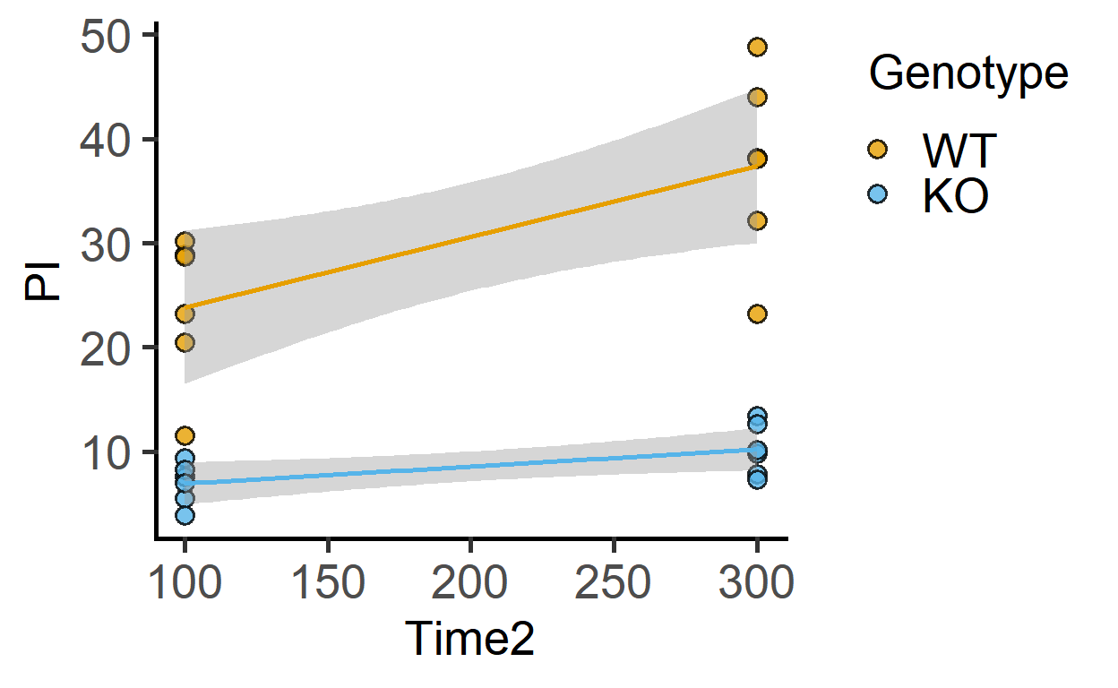
The above plot is not possible with the Time variable, which is a categorical factor, and was used with plot_4d_scatterbox, for example.
We can use posthoc_Trends on a linear model fit using Time2 as numeric covariate to assess difference in slopes and values at different time points.
#fit a model with Time2

tmod <- mixed_model(data_2w_Tdeath,
                    "PI",
                    c("Genotype", "Time2"),
                    "Experiment")
#get slopes (trends) of lines and their comparisons
#there are only 2 levels in Genotype
#all these give same results

posthoc_Trends_Pairwise(Model = tmod,
                        Fixed_Factor = "Genotype",
                        Trend_Factor = "Time2")
#> $emtrends
#> Genotype Time2.trend SE df lower.CL upper.CL
#> WT 0.0678 0.0144 15 0.0371 0.0985
#> KO 0.0163 0.0144 15 -0.0144 0.0471
#>
#> Results are averaged over the levels of: Time2
#> Degrees-of-freedom method: kenward-roger
#> Confidence level used: 0.95
#>
#> $contrasts
#> contrast estimate SE df t.ratio p.value
#> WT - KO 0.0515 0.0204 15 2.526 0.0233
#>
#> Results are averaged over the levels of: Time2
#> Degrees-of-freedom method: kenward-rogerposthoc_Trends_Levelwise(Model = tmod,
Fixed_Factor = c("Genotype", "Time2"),
Trend_Factor = "Time2")#> $emtrends
#> Time2 = 100:
#> Genotype Time2.trend SE df lower.CL upper.CL
#> WT 0.0678 0.0144 15 0.0371 0.0985
#> KO 0.0163 0.0144 15 -0.0144 0.0471
#>
#> Time2 = 300:
#> Genotype Time2.trend SE df lower.CL upper.CL
#> WT 0.0678 0.0144 15 0.0371 0.0985
#> KO 0.0163 0.0144 15 -0.0144 0.0471
#>
#> Degrees-of-freedom method: kenward-roger
#> Confidence level used: 0.95
#>
#> $contrasts
#> Time2 = 100:
#> contrast estimate SE df t.ratio p.value
#> WT - KO 0.0515 0.0204 15 2.526 0.0233
#>
#> Time2 = 300:
#> contrast estimate SE df t.ratio p.value
#> WT - KO 0.0515 0.0204 15 2.526 0.0233
#>
#> Degrees-of-freedom method: kenward-rogerposthoc_Trends_vsRef(Model = tmod,
Fixed_Factor = c("Genotype", "Time2"),
Trend_Factor = "Time2",
Ref_Level = 2) #WT is level 2#> $emtrends
#> Time2 = 100:
#> Genotype Time2.trend SE df lower.CL upper.CL
#> WT 0.0678 0.0144 15 0.0371 0.0985
#> KO 0.0163 0.0144 15 -0.0144 0.0471
#>
#> Time2 = 300:
#> Genotype Time2.trend SE df lower.CL upper.CL
#> WT 0.0678 0.0144 15 0.0371 0.0985
#> KO 0.0163 0.0144 15 -0.0144 0.0471
#>
#> Degrees-of-freedom method: kenward-roger
#> Confidence level used: 0.95
#>
#> $contrasts
#> Time2 = 100:
#> contrast estimate SE df t.ratio p.value
#> WT - KO 0.0515 0.0204 15 2.526 0.0233
#>
#> Time2 = 300:
#> contrast estimate SE df t.ratio p.value
#> WT - KO 0.0515 0.0204 15 2.526 0.0233
#>
#> Degrees-of-freedom method: kenward-roger