Two functions are available for fitting a basic type of generalised additive model (GAM). Please see other resources for an introduction to the mgcv package and the use of GAMs (here by Kim Larsen, Michael Clarke, and the use of random effects with gam.
These page documents functions for GAMs to provide the:
- ANOVA table (
ga_anova). - Fitted model (
ga_model), which is useful for diagnostics and posthoc comparisons. - Diagnostics and plotting predictions (
model_qq_gam,plot_gam_predict).
Both ga_model and ga_anova use the factor by fit with a one smooth term (e.g., time) and one categorical variable with multiple levels (e.g. Genotype as WT and KO, or Treatment as ‘untreated’ and ‘treated’).
Data format
See the data help page and ensure data table is in the long-format, and check that you have correctly converted categorical variables with as.factor and columns with numeric variables are in the correct format. These functions can be used for fitting linear models on continuous predictors (e.g. time). Note that post-hoc comparisons for slopes and intercepts can be run with emtrends from the emmeans package.
Fitting a GAM
This examples uses the data_zooplanton data that contains the dependent numeric variable density_adj which was measured across time (numeric independent variable day with many levels), for zooplankton of four taxa (a categorical variable taxon with 4 levels). These are data from measurements of these taxa at four lakes (a categorical variable with 4 levels) over several years.
head(data_zooplankton, n = 5) #see first 5 rows#> day year lake taxon density density_adj min_density
#> 37 16 1984 Menona Calanoid copepods 0 0.1 2000
#> 40 16 1984 Menona D. thomasi 21000 2.2 2000
#> 41 16 1984 Menona K. cochlearis 11000 1.2 2000
#> 42 16 1984 Menona L. siciloides 49000 5.0 2000
#> 61 20 1976 Menona Calanoid copepods 64000 6.5 2000
#> density_scaled
#> 37 -1.7040700
#> 40 0.3450740
#> 41 -2.0580472
#> 42 -0.5145089
#> 61 0.2250025str(data_zooplankton) #check data frame structure#> 'data.frame': 1127 obs. of 8 variables:
#> $ day : int 16 16 16 16 20 20 20 20 20 20 ...
#> $ year : int 1984 1984 1984 1984 1976 1976 1976 1976 1987 1987 ...
#> $ lake : Factor w/ 4 levels "Kegonsa","Mendota",..: 3 3 3 3 3 3 3 3 3 3 ...
#> $ taxon : Factor w/ 8 levels "C. sphaericus",..: 2 5 6 7 2 5 6 7 2 5 ...
#> $ density : num 0 21000 11000 49000 64000 43000 0 64000 0 78000 ...
#> $ density_adj : num 0.1 2.2 1.2 5 6.5 4.4 0.1 6.5 0.1 7.9 ...
#> $ min_density : int 2000 2000 2000 2000 2000 2000 2000 2000 2000 2000 ...
#> $ density_scaled: num -1.704 0.345 -2.058 -0.515 0.225 ...#fit the model
zooGAM1 <- ga_model(data_zooplankton,
"density_adj",
"taxon",
"day")
#diagnostic plots
plot_qq_gam(zooGAM1)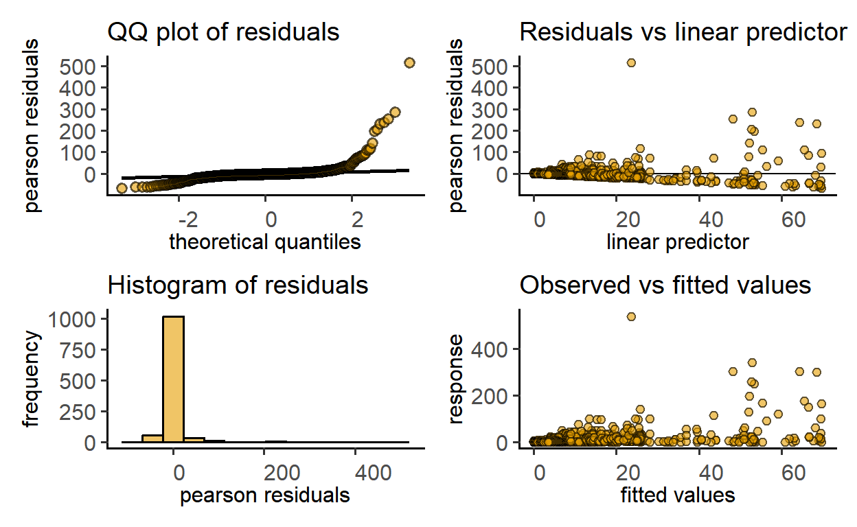
The output indicates a bad fit, which could be improved with a log-transformation of the dependent variable.
#log-transformed data model
zooGAM2 <- ga_model(data_zooplankton,
                    "log(density_adj)",
                    "taxon",
                    "day")
#diagnostic plots
plot_qq_gam(zooGAM2)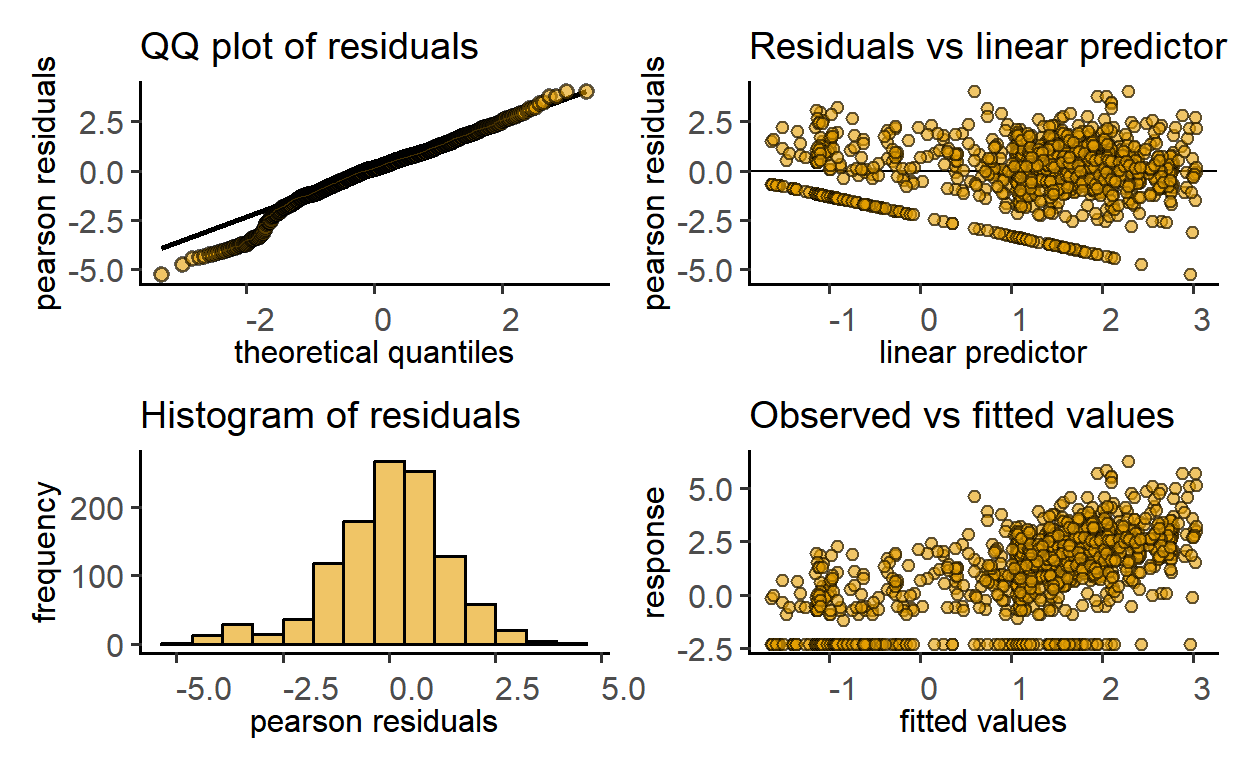
ANOVA table of above model
#with the ga_anova function
ga_anova(data_zooplankton,
         "log(density_adj)",
         "taxon",
         "day")
#>
#> Family: gaussian
#> Link function: identity
#>
#> Formula:
#> log(density_adj) ~ taxon + s(day, by = taxon)
#>
#> Parametric Terms:
#> df F p-value
#> taxon 3 23.97 4.97e-15
#>
#> Approximate significance of smooth terms:
#> edf Ref.df F p-value
#> s(day):taxonCalanoid copepods 7.828 8.643 28.267 < 2e-16
#> s(day):taxonD. thomasi 6.989 8.057 42.695 < 2e-16
#> s(day):taxonK. cochlearis 5.349 6.470 5.739 5.76e-06
#> s(day):taxonL. siciloides 3.076 3.825 5.322 0.000466#or anova call on fitted model
anova(zooGAM2)#>
#> Family: gaussian
#> Link function: identity
#>
#> Formula:
#> log(density_adj) ~ taxon + s(day, by = taxon)
#>
#> Parametric Terms:
#> df F p-value
#> taxon 3 23.97 4.97e-15
#>
#> Approximate significance of smooth terms:
#> edf Ref.df F p-value
#> s(day):taxonCalanoid copepods 7.828 8.643 28.267 < 2e-16
#> s(day):taxonD. thomasi 6.989 8.057 42.695 < 2e-16
#> s(day):taxonK. cochlearis 5.349 6.470 5.739 5.76e-06
#> s(day):taxonL. siciloides 3.076 3.825 5.322 0.000466Plot model predictions
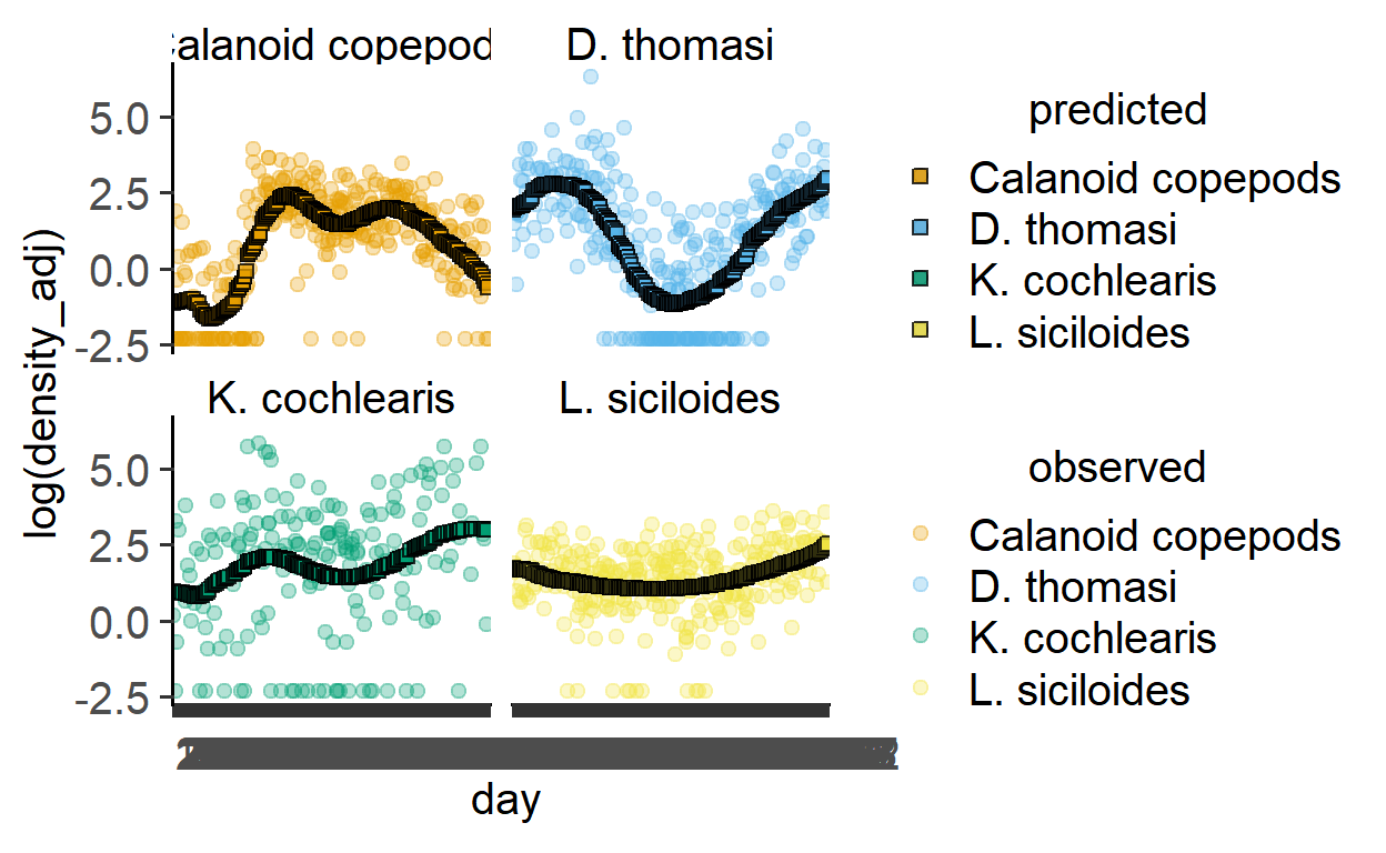
There is a dedicated function to plot predictions of GAMs (plot_gam_predict).
plot_gam_predict(zooGAM2,
                 day,
                 `log(density_adj)`,
                 taxon)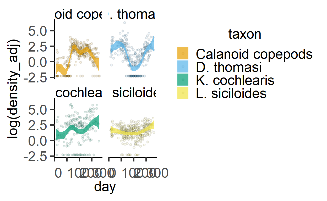
The plot_lm_predict can also be used.
plot_lm_predict(zooGAM2,
                day,
                `log(density_adj)`,
                taxon)