Six functions are available for fitting linear models or linear mixed effects models. They rely on lm and lmer (latter implemented in package lmerTest).
This page documents functions for simple (ordinary) linear models to provide the:
- ANOVA table (
simple_anova) with F and P values - Fitted model (
simple_model), which is useful for diagnostics and posthoc comparisons.
Both fit the full model with interaction terms when more than one fixed factors are provided.
Type II SS
ANOVA tables show type II sum of squares. ANOVA tables with simple_anova are generated using the car::Anova() call.
If you want Type III SS, first set contrasts using options(contrasts=c("contr.sum", "contr.poly") before fitting the model or getting the ANOVA table. Fitting the model without this and setting type = "III" will give incorrect results. The default contrasts in R can be obtained by running options(contrasts=c("contr.treatment", "contr.poly")).
Data format
See the data help page and ensure data table is in the long-format, and check that you have correctly converted categorical variables with as.factor and columns with numeric variables are in the correct format.
Examples used here
We will use data_1w_death and data_2w_Festing in these examples. In this vignette we use ordinary linear models; see the vignette on mixed-effects models for analyses of the same data where the random factor is taken into account.
Let’s look at these data first so you have an idea of whether or not there are differences between them.
First the data_1w_death (one-way ANOVA design) data from 5 independent in vitro experiments where death of host cells was measured (as percentage of total cells) after infection with three different strains of a pathogenic bacterium (factor Genotype).
head(data_1w_death, n = 6) #see first 6 rows of data#> Experiment Genotype Death
#> 1 Exp_1 WT 25.012173
#> 2 Exp_1 KO_1 1.824973
#> 3 Exp_1 KO_2 14.294956
#> 4 Exp_2 WT 16.542609
#> 5 Exp_2 KO_1 2.131199
#> 6 Exp_2 KO_2 23.749439A plot of these data shows that KO_1 induces very little death as compared to the other two bacterial strains.
plot_3d_scatterbox(data_1w_death, #data
                   Genotype,      #fixed factor
                   Death,         #Y variable
                   Genotype)      #shapes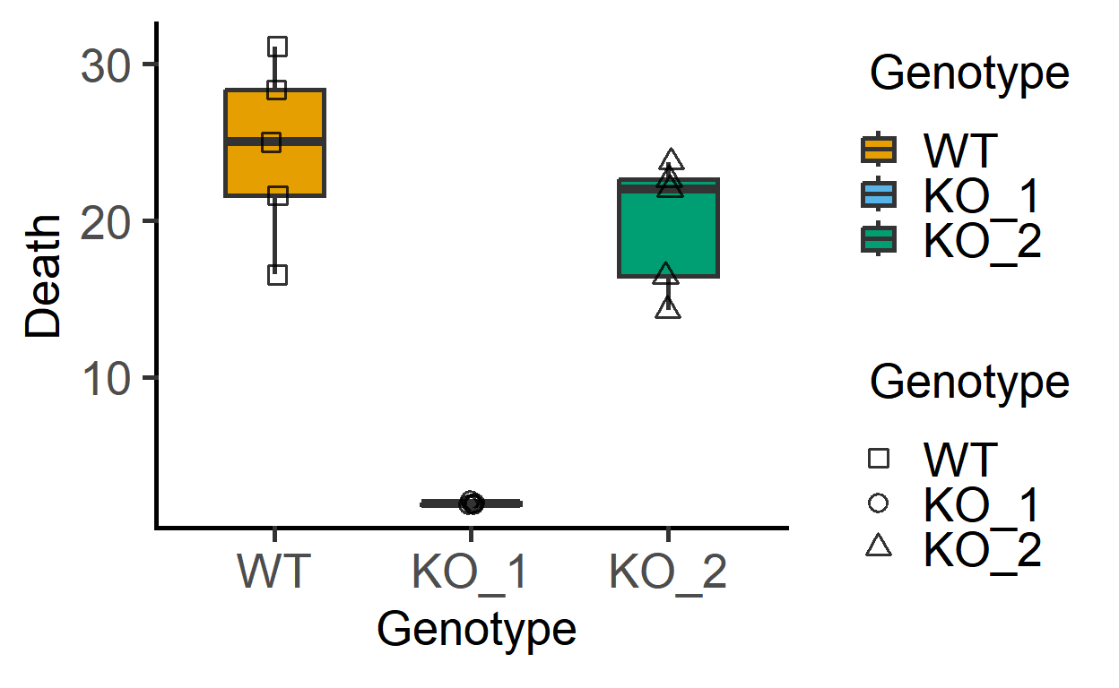
The data_2w_Festing data from Festing et al dataset has two fixed factors (“Treatment” & “Strain”). For the present analysis, I will ignore the blocking factor (“Block”), and we use the same data set in the vignette on mixed effects models (mixed_anova).
head(data_2w_Festing, n = 8) #see first 8 rows#> Block Treatment Strain GST
#> 1 A Control NIH 444
#> 2 A Treated NIH 614
#> 3 A Control BALB/C 423
#> 4 A Treated BALB/C 625
#> 5 A Control A/J 408
#> 6 A Treated A/J 856
#> 7 A Control 129/Ola 447
#> 8 A Treated 129/Ola 719The plot below of these data suggests that Treatment generally increases GST values irrespective of the mouse Strain (although the magnitude of increase appears to be different across the strains).
plot_4d_scatterbox(data_2w_Festing, #data
                   Strain,          #factor 1
                   GST,             #Y  variable
                   Treatment,       #factor 2
                   Treatment)       #shapes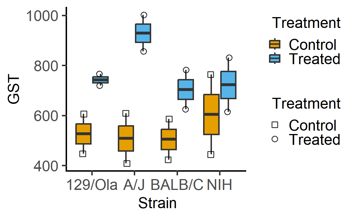
Let’s fit a linear model, use diagnostics and get ANOVA table.
simple_model
In general, you should first fit a linear model, perform diagnostics on the model and then proceed to getting an ANOVA table and post-hoc comparisons.
This function generates a fitted model (you need to explicitly save this object), which will be required for model diagnostics and post-hoc comparisons using posthoc_ functions – see separate the posthoc_ vignette.
sm_death <- simple_model(data_1w_death, #data
                         "Death",       #Y variable
                         "Genotype")    #Fixed factor
Get the summary of the model using summary(). The summary shows the formula used to fit the linear model at the top.
summary(sm_death) #>
#> Call:
#> lm(formula = Death ~ Genotype, data = data_1w_death)
#>
#> Residuals:
#> Min 1Q Median 3Q Max
#> -7.9834 -1.5226 0.0159 2.4960 6.5997
#>
#> Coefficients:
#> Estimate Std. Error t value Pr(>|t|)
#> (Intercept) 24.526 1.830 13.403 1.40e-08 ***
#> GenotypeKO_1 -22.586 2.588 -8.727 1.53e-06 ***
#> GenotypeKO_2 -4.699 2.588 -1.816 0.0945 .
#> ---
#> Signif. codes: 0 '***' 0.001 '**' 0.01 '*' 0.05 '.' 0.1 ' ' 1
#>
#> Residual standard error: 4.092 on 12 degrees of freedom
#> Multiple R-squared: 0.8761, Adjusted R-squared: 0.8554
#> F-statistic: 42.41 on 2 and 12 DF, p-value: 3.624e-06Check model residuals with the plot_qqmodel function.
plot_qqmodel(sm_death) #sm_dtime saved above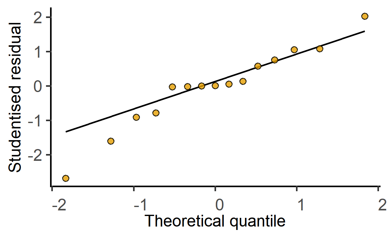
Factorial designs can be analysed by providing fixed factors as a vector. A full model with interactions will be fit.
sm2 <- simple_model(data_2w_Festing,    #data
                    "GST",              #Y variable
                    c("Strain", "Treatment"))   #Fixed factors as a vector

#get model summary
summary(sm2)
#>
#> Call:
#> lm(formula = GST ~ Strain * Treatment, data = data_2w_Festing)
#>
#> Residuals:
#> Min 1Q Median 3Q Max
#> -160 -80 0 80 160
#>
#> Coefficients:
#> Estimate Std. Error t value Pr(>|t|)
#> (Intercept) 526.50 95.18 5.531 0.000553
#> StrainA/J -18.00 134.61 -0.134 0.896926
#> StrainBALB/C -22.00 134.61 -0.163 0.874228
#> StrainNIH 77.50 134.61 0.576 0.580620
#> TreatmentTreated 216.00 134.61 1.605 0.147239
#> StrainA/J:TreatmentTreated 204.50 190.37 1.074 0.314042
#> StrainBALB/C:TreatmentTreated -17.00 190.37 -0.089 0.931037
#> StrainNIH:TreatmentTreated -97.50 190.37 -0.512 0.622368
#>
#> (Intercept) ***
#> StrainA/J
#> StrainBALB/C
#> StrainNIH
#> TreatmentTreated
#> StrainA/J:TreatmentTreated
#> StrainBALB/C:TreatmentTreated
#> StrainNIH:TreatmentTreated
#> ---
#> Signif. codes: 0 '***' 0.001 '**' 0.01 '*' 0.05 '.' 0.1 ' ' 1
#>
#> Residual standard error: 134.6 on 8 degrees of freedom
#> Multiple R-squared: 0.6784, Adjusted R-squared: 0.3969
#> F-statistic: 2.41 on 7 and 8 DF, p-value: 0.1205#qq plot of model residuals
plot_qqmodel(sm2)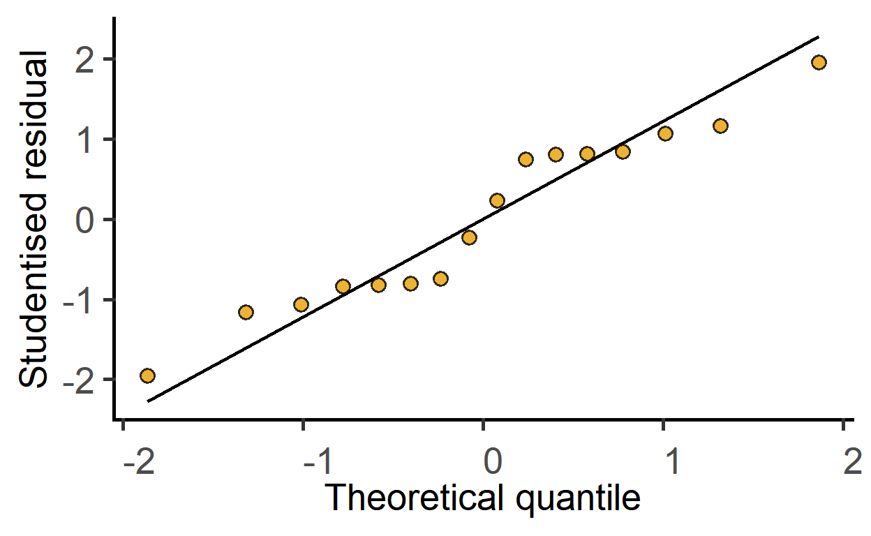
The ggResidPanel package is great for model diagnostics. Check it out.
simple_anova
Use this function for ordinary ANOVA designs without a random factor. Repeated-measures cannot be analysed at present; use mixed_anova instead with a column indicating repeated-measured IDs/factors. The arguments for this function are identical to simple_model. anova() call on model objects will produce similar results.
One-way ANOVA
Let’s get the ANOVA table from an ordinary one-way ANOVA design data with three groups with the data_1w_death data used above.
simple_anova(data = data_1w_death,  #data
             Y_value = "Death",     #Y variable
             Fixed_Factor = "Genotype") #Fixed factor
#> Anova Table (Type II tests)
#>
#> Response: Death
#> Sum Sq Mean sq Df F value Pr(>F)
#> Genotype 1420.21 710.10 2 42.412 3.624e-06 ***
#> Residuals 200.91 16.74 12
#> ---
#> Signif. codes: 0 '***' 0.001 '**' 0.01 '*' 0.05 '.' 0.1 ' ' 1The large F value (42.412) & small P value (3.6e-06) suggest major difference between levels of Genotypes.
Two-way ANOVA
For more than one fixed factors, provide them as a vector to the Fixed_Factor argument.
simple_anova(data_2w_Festing,           #data
             "GST",                     #Y variable
             c("Strain", "Treatment"))  #fixed factors as a vector
#> Anova Table (Type II tests)
#>
#> Response: GST
#> Sum Sq Mean sq Df F value Pr(>F)
#> Strain 28613 9538 3 0.5264 0.67640
#> Treatment 227529 227529 1 12.5570 0.00758 **
#> Strain:Treatment 49591 16530 3 0.9123 0.47705
#> Residuals 144957 18120 8
#> ---
#> Signif. codes: 0 '***' 0.001 '**' 0.01 '*' 0.05 '.' 0.1 ' ' 1This suggest an effect of Treatment and no impact of Strain, and no interaction.
Data transformations
Common data transformations are possible, such as log-transformation if you want to compare ratios.
simple_anova(data_2w_Festing,           #data
             "log(GST)",                 #log-transfored Y variable
             c("Strain", "Treatment"))   #fixed factors as a vector
#> Anova Table (Type II tests)
#>
#> Response: log(GST)
#> Sum Sq Mean sq Df F value Pr(>F)
#> Strain 0.04263 0.01421 3 0.2758 0.84139
#> Treatment 0.57596 0.57596 1 11.1772 0.01018 *
#> Strain:Treatment 0.09056 0.03019 3 0.5858 0.64106
#> Residuals 0.41224 0.05153 8
#> ---
#> Signif. codes: 0 '***' 0.001 '**' 0.01 '*' 0.05 '.' 0.1 ' ' 1#see the difference in SumSq, MeanSq etc.
#because of log transformation, ratios are being comparedPlotting model-predicted data
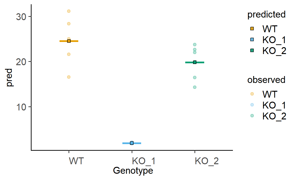
The function plot_lm_predict is handy to check how close the values predicted from the linear model are to observed (or measured) values that were used to fit the model. A good model will predict numbers close to observed/real data.
This function takes in a fitted model, and needs X and Y variables that exactly match those used to fit the model.
Let us plot the predictions of models fitted above.
plot_lm_predict(Model = sm2,   #fitted model
                xcol = Strain, #one independent factor
                ycol = GST)    #dependent numeric factor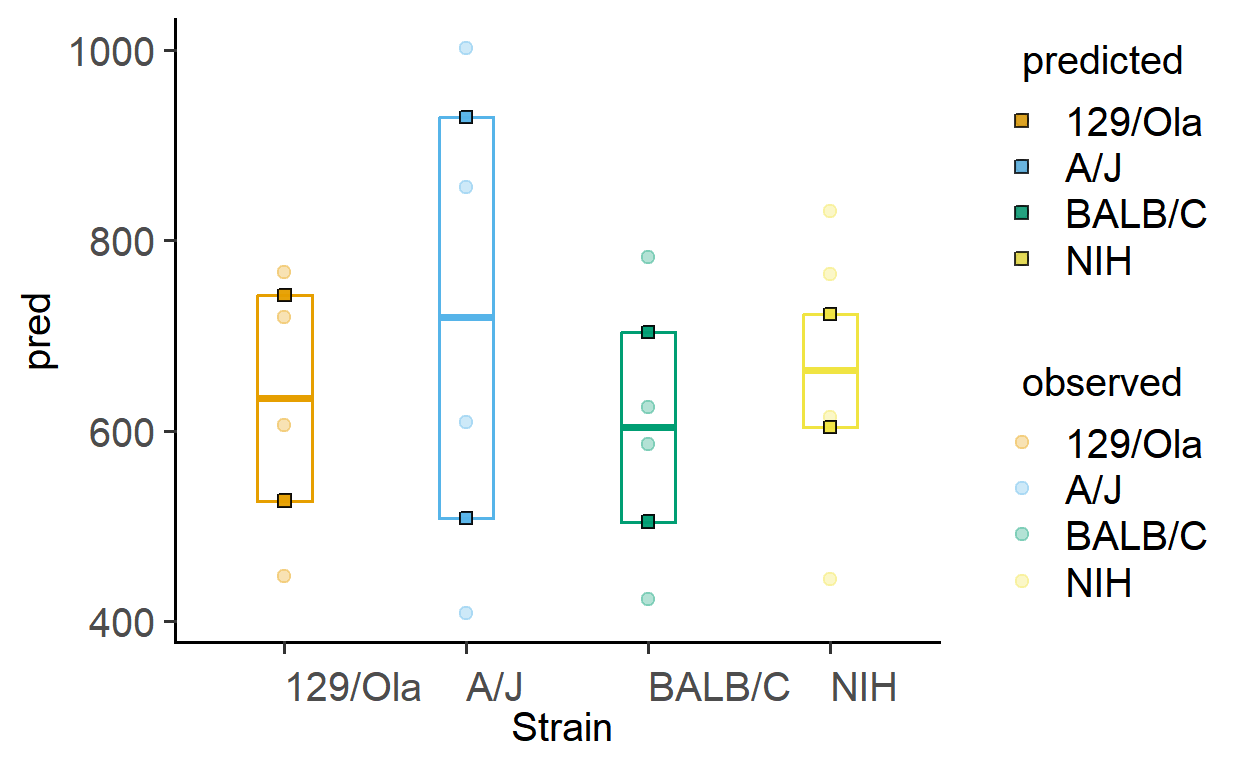
plot_lm_predict(Model = sm_death, #fitted model
                xcol = Genotype,   #one independent factor
                ycol = Death)  #dependent numeric factor